3 Practice

3.1 Introduction to forecasting practice⁹¹

The purpose of forecasting is to improve decision making in the face of uncertainty. To achieve this, forecasts should provide an unbiased guess at what is most likely to happen (the point forecast), along with a measure of uncertainty, such as a prediction interval (PI). Such information will facilitate appropriate decisions and actions.

Forecasting should be an objective, dispassionate exercise, one that is built upon facts, sound reasoning, and sound methods. But since forecasts are created in social settings, they are influenced by organisational politics and personal agendas. As a consequence, forecasts will often reflect aspirations rather than unbiased projections.

In organisations, forecasts are created through processes that can involve multiple steps and participants. The process can be as simple as executive fiat (also known as evangelical forecasting), unencumbered by what the data show. More commonly, the process begins with a statistical forecast (generated by forecasting software), which is then subject to review and adjustment, as illustrated in Figure 5.

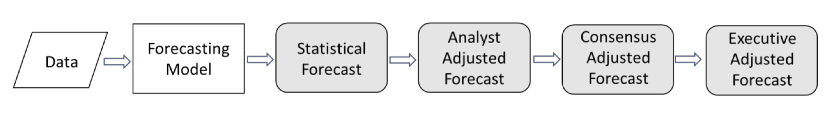
Figure 5: Multi-stage forecasting process.

In concept, such an elaborate multi-stage process allows “management intelligence” to improve forecast quality, incorporating information not accounted for in the statistical model. In reality, however, benefits are not assured. Lawrence, Goodwin, O’Connor, & Önkal (2006) reviewed more than 200 studies, concluding that human judgment can be of significant benefit but is also subject to significant biases. Among the many papers on this subject, there is general agreement on the need to track and review overrides, and the need to better understand the psychological issues around judgmental adjustments.

The underlying problem is that each human touch point subjects the forecast to the interests of the reviewers – and these interests may not align with creating an accurate, unbiased forecast. To identify where such problems are occurring, Forecast Value Added (FVA) analysis is an increasingly popular approach among practitioners.

FVA is defined as the change in a forecasting performance metric that can be attributed to a particular step or participant in the forecasting process (Gilliland, 2002). Any activity that fails to deliver positive FVA (i.e., fails to improve forecast quality) is considered process waste.

Starting with a naive forecast, FVA analysis seeks to determine whether each subsequent step in the process improves upon the prior steps. The “stairstep report” of Table 1 is a familiar way of summarising results, as in this example from Newell Rubbermaid (Schubert & Rickard, 2011).

Table 1: Stairstep report showing FVA results.

Process Step	Forecast accuracy (100%\(-\)MAPE)	FVA vs. Naive	FVA vs. Statistical
Naive forecast	60%
Statistical forecast	65%	5%
Adjusted forecast	62%	2%	-3%

Here, averaged across all products, naive (random walk) achieved forecast accuracy of 60%. The company’s statistical forecast delivered five percentage points of improvement, but management review and adjustment delivered negative value. Such findings – not uncommon – urge further investigation into causes and possible process corrections (such as training reviewers or limiting adjustments). Alternatively, the management review step could be eliminated, providing the dual benefits of freeing up management time spent on forecasting and, on average, more accurate forecasts.

Morlidge (2014c) expanded upon FVA analysis to present a strategy for prioritising judgmental adjustments, finding the greatest opportunity for error reduction in products with high volume and high relative absolute error. Chase (2021) described a machine learning (ML) method to guide forecast review, identifying which forecasts are most likely to benefit from adjustment along with a suggested adjustment range. Baker (2021) used ML classification models to identify characteristics of non-value adding overrides, proposing the behavioural economics notion of a “nudge” to prompt desired forecaster behaviour. Further, Goodwin, Petropoulos, & Hyndman (2017) derived upper bounds for FVA relative to naive forecasts. And Kok (2017) created a Stochastic Value Added (SVA) metric to assess the difference between actual and forecasted distributions, knowledge of which is valuable for inventory management.

Including an indication of uncertainty around the point forecast remains an uncommon practice. Prediction intervals in software generally underestimate uncertainty, often dramatically, leading to unrealistic confidence in the forecast. And even when provided, PIs largely go unused by practitioners. Goodwin (2014) summarised the psychological issues, noting that the generally poor calibration of the PIs may not explain the reluctance to utilise them. Rather, “an interval forecast may accurately reflect the uncertainty, but it is likely to be spurned by decision makers if it is too wide and judged to be uninformative” (Goodwin, 2014, p. 5).

It has long been recognised (Chatfield, 1986; Lawrence, 2000) that the practice of forecasting falls well short of the potential exhibited in academic research, and revealed by the M forecasting competitions. In the M4, a simple benchmark combination method (the average of Single, Holt, and Damped exponential smoothing) reduced the overall weighted average (OWA) error by 17.9% compared to naive. The top six performing methods in M4 further reduced OWA by over 5% compared to the combination benchmark (Makridakis et al., 2020b). But in forecasting practice, just bettering the accuracy of naive has proven to be a surprising challenge. Morlidge (2014b)’s study of eight consumer and industrial businesses found 52% of their forecasts failed to do so. And, as shown, Newel Rubbermaid beat naive by just two percentage points after management adjustments.

Ultimately, forecast accuracy is limited by the nature of the behaviour being forecast. But even a highly accurate forecast is of little consequence if overridden by management and not used to enhance decision making and improve organisational performance.

Practitioners need to recognise limits to forecastability and be willing to consider alternative (non-forecasting) approaches when the desired level of accuracy is not achievable (Gilliland, 2010). Alternatives include supply chain re-engineering – to better react to unforeseen variations in demand, and demand smoothing – leveraging pricing and promotional practices to shape more favourable demand patterns.

Despite measurable advances in our statistical forecasting capabilities (Spyros Makridakis et al., 2020a), it is questionable whether forecasting practice has similarly progressed. The solution, perhaps, is what Morlidge (2014a) (page 39) suggests that “users should focus less on trying to optimise their forecasting process than on detecting where their process is severely suboptimal and taking measures to redress the problem”. This is where FVA can help.

For now, the challenge for researchers remains: To prompt practitioners to adopt sound methods based on the objective assessment of available information, and avoid the “worst practices” that squander resources and fail to improve the forecast.

3.2 Operations and supply chain management

3.2.1 Demand management⁹²

Demand management is one of the dominant components of supply chain management (Fildes, Goodwin, & Lawrence, 2006). Accurate demand estimate of the present and future is a first vital step for almost all aspects of supply chain optimisation, such as inventory management, vehicle scheduling, workforce planning, and distribution and marketing strategies (Kolassa & Siemsen, 2016). Simply speaking, better demand forecasts can yield significantly better supply chain management, including improved inventory management and increased service levels. Classic demand forecasts mainly rely on qualitative techniques, based on expert judgment and past experience (e.g., Weaver, 1971), and quantitative techniques, based on statistical and machine learning modelling (e.g., James W Taylor, 2003b; Bacha & Meyer, 1992). A combination of qualitative and quantitative methods is also popular and proven to be beneficial in practice by, e.g., judgmental adjustments (Önkal & Gönül, 2005; Aris A Syntetos et al., 2016b and §2.11.2; Turner, 1990), judgmental forecast model selection (Han et al., 2019 and §2.11.3; Petropoulos et al., 2018b), and other advanced forecasting support systems (Arvan, Fahimnia, Reisi, & Siemsen, 2019 see also §3.7.1; Baecke, De Baets, & Vanderheyden, 2017).

The key challenges that demand forecasting faces vary from domain to domain. They include:

1. The existence of intermittent demands, e.g., irregular demand patterns of fashion products. According to Nikolopoulos (2020), limited literature has focused on intermittent demand. The seminal work by Croston (1972) was followed by other representative methods such as the SBA method by Syntetos & Boylan (2001), the aggregate–disaggregate intermittent demand approach (ADIDA) by Nikolopoulos et al. (2011), the multiple temporal aggregation by Petropoulos & Kourentzes (2015), and the \(k\) nearest neighbour (\(k\)NN) based approach by Nikolopoulos et al. (2016). See §2.8 for more details on intermittent demand forecasting and §2.10.2 for a discussion on temporal aggregation.

2. The emergence of new products. Recent studies on new product demand forecasting are based on finding analogies (Hu, Acimovic, Erize, Thomas, & Van Mieghem, 2019; Wright & Stern, 2015), leveraging comparable products (Baardman, Levin, Perakis, & Singhvi, 2018), and using external information like web search trends (Kulkarni, Kannan, & Moe, 2012). See §3.2.6 for more details on new product demand forecasting.

3. The existence of short-life-cycle products, e.g., smartphone demand (e.g., Szozda, 2010; Chung, Niu, & Sriskandarajah, 2012; Shi et al., 2020).

4. The hierarchical structure of the data such as the electricity demand mapped to a geographical hierarchy (e.g., Athanasopoulos et al., 2009; Hong et al., 2019 but also §2.10.1; Hyndman et al., 2011).

With the advent of the big data era, a couple of coexisting new challenges have drawn the attention of researchers and practitioners in the forecasting community: the need to forecast a large volume of related time series (e.g., thousands or millions of products from one large retailer: Salinas et al., 2019a), and the increasing number of external variables that have significant influence on future demand (e.g., massive amounts of keyword search indices that could impact future tourism demand (Law, Li, Fong, & Han, 2019)). Recently, to deal with these new challenges, numerous empirical studies have identified the potentials of deep learning based global models, in both point and probabilistic demand forecasting (e.g., Wen et al., 2017; Bandara et al., 2020b; Rangapuram et al., 2018; Salinas et al., 2019a). With the merits of cross-learning, global models have been shown to be able to learn long memory patterns and related effects (Montero-Manso & Hyndman, 2020), latent correlation across multiple series (Smyl, 2020), handle complex real-world forecasting situations such as data sparsity and cold-starts (Chen, Kang, Chen, & Wang, 2020), include exogenous covariates such as promotional information and keyword search indices (Law et al., 2019), and allow for different choices of distributional assumptions (Salinas et al., 2019a).

3.2.2 Forecasting in the supply chain⁹³

A supply chain is ‘a network of stakeholders (e.g., retailers, manufacturers, suppliers) who collaborate to satisfy customer demand’ (Perera et al., 2019). Forecasts inform many supply chain decisions, including those relating to inventory control, production planning, cash flow management, logistics and human resources (also see §3.2.1). Typically, forecasts are based on an amalgam of statistical methods and management judgment (Fildes & Goodwin, 2007). Hofmann & Rutschmann (2018) have investigated the potential for using big data analytics in supply chain forecasting but indicate more research is needed to establish its usefulness.

In many organisations forecasts are a crucial element of Sales and Operations Planning (S&OP), a tool that brings together different business plans, such as those relating to sales, marketing, manufacturing and finance, into one integrated set of plans (Thomé, Scavarda, Fernandez, & Scavarda, 2012). The purposes of S&OP are to balance supply and demand and to link an organisation’s operational and strategic plans. This requires collaboration between individuals and functional areas at different levels because it involves data sharing and achieving a consensus on forecasts and common objectives (Mello, 2010). Successful implementations of S&OP are therefore associated with forecasts that are both aligned with an organisation’s needs and able to draw on information from across the organisation. This can be contrasted with the ‘silo culture’ identified in a survey of companies by Moon, Mentzer, & Smith (2003) where separate forecasts were prepared by different departments in ‘islands of analysis’. Methods for reconciling forecasts at different levels in both cross-sectional hierarchies (e.g., national, regional and local forecasts) and temporal hierarchies (e.g., annual, monthly and daily forecasts) are also emerging as an approach to break through information silos in organisations (see §2.10.1, §2.10.2, and §2.10.3). Cross-temporal reconciliation provides a data-driven approach that allows information to be drawn from different sources and levels of the hierarchy and enables this to be blended into coherent forecasts (Kourentzes & Athanasopoulos, 2019).

In some supply chains, companies have agreed to share data and jointly manage planning processes in an initiative known as Collaborative Planning, Forecasting, and Replenishment (CPFR) (Seifert, 2003 also see §3.2.3). CPFR involves pooling information on inventory levels and on forthcoming events, like sales promotions. Demand forecasts can be shared, in real time via the Internet, and discrepancies between them reconciled. In theory, information sharing should reduce forecast errors. This should mitigate the ‘bullwhip effect’ where forecast errors at the retail-end of supply chains cause upstream suppliers to experience increasingly volatile demand, forcing them to hold high safety stock levels (Lee et al., 2007). Much research demonstrating the benefits of collaboration has involved simulated supply chains (Fildes, 2017). Studies of real companies have also found improved performance through collaboration (e.g., Boone & Ganeshan, 2008; Eksoz, Mansouri, Bourlakis, & Önkal, 2019; Hill, Zhang, & Miller, 2018), but case study evidence is still scarce (Aris A Syntetos et al., 2016a). The implementation of collaborative schemes has been slow with many not progressing beyond the pilot stage (Galbreth, Kurtuluş, & Shor, 2015; Panahifar, Byrne, & Heavey, 2015). Barriers to successful implementation include a lack of trust between organisations, reward systems that foster a silo mentality, fragmented forecasting systems within companies, incompatible systems, a lack of relevant training and the absence of top management support (Fliedner, 2003; Thomé, Hollmann, & Scavarda do Carmo, 2014).

Initiatives to improve supply chain forecasting can be undermined by political manipulation of forecasts and gaming. Examples include ‘enforcing’: requiring inflated forecasts to align them with sales or financial goals, ‘sandbagging’: underestimating sales so staff are rewarded for exceeding forecasts, and ‘spinning’: manipulating forecasts to garner favourable reactions from colleagues (Mello, 2009). Pennings, Dalen, & Rook (2019) discuss schemes for correcting such intentional biases.

For a discussion of the forecasting of returned items in supply chains, see §3.2.9, while §3.9 offers a discussion of possible future developments in supply chain forecasting.

3.2.3 Forecasting for inventories⁹⁴

Three aspects of the interaction between forecasting and inventory management have been studied in some depth and are the subject of this review: the bullwhip effect, forecast aggregation, and performance measurement.

The ‘bullwhip effect’ occurs whenever there is amplification of demand variability through the supply chain (Lee, Padmanabhan, & Whang, 2004), leading to excess inventories. This can be addressed by supply chain members sharing downstream demand information, at stock keeping unit level, to take advantage of less noisy data. Analytical results on the translation of ARIMA (see §2.3.4) demand processes have been established for order-up-to inventory systems (Gilbert, 2005). There would be no value in information sharing if the wholesaler can use such relationships to deduce the retailer’s demand process from their orders (see, for example, Graves, 1999). Such deductions assume that the retailer’s demand process and demand parameters are common knowledge to supply chain members. Ali & Boylan (2011) showed that, if such common knowledge is lacking, there is value in sharing the demand data itself and Ali, Boylan, & Syntetos (2012) established relationships between accuracy gains and inventory savings. Analytical research has tended to assume that demand parameters are known. Pastore, Alfieri, Zotteri, & Boylan (2020) investigated the impact of demand parameter uncertainty, showing how it exacerbates the bullwhip effect.

Forecasting approaches have been developed that are particularly suitable in an inventory context, even if not originally proposed to support inventory decisions. For example, Nikolopoulos et al. (2011) proposed that forecasts could be improved by aggregating higher frequency data into lower frequency data (see also §2.10.2; other approaches are reviewed in §3.2.1). Following this approach, Forecasts are generated at the lower frequency level and then disaggregated, if required, to the higher frequency level. For inventory replenishment decisions, the level of aggregation may conveniently be chosen to be the lead time, thereby taking advantage of the greater stability of data at the lower frequency level, with no need for disaggregation.

The variance of forecast errors over lead time is required to determine safety stock requirements for continuous review systems. The conventional approach is to take the variance of one-step-ahead errors and multiply it by the lead time. However, this estimator is unsound, even if demand is independent and identically distributed, as explained by Prak, Teunter, & Syntetos (2017). A more direct approach is to smooth the mean square errors over the lead time (Syntetos & Boylan, 2006).

Strijbosch & Moors (2005) showed that unbiased forecasts will not necessarily lead to achievement, on average, of target cycle service levels or fill rates. Wallström & Segerstedt (2010) proposed a ‘Periods in Stock’ measure, which may be interpreted, based on a ‘fictitious stock’, as the number of periods a unit of the forecasted item has been in stock or out of stock. Such measures may be complemented by a detailed examination of error-implication metrics (Boylan & Syntetos, 2006). For inventory management, these metrics will typically include inventory holdings and service level implications (e.g., cycle service level, fill rate). Comparisons may be based on total costs or via ‘exchange curves’, showing the trade-offs between service and inventory holding costs. Comparisons such as these are now regarded as standard in the literature on forecasting for inventories and align well with practice in industry.

3.2.4 Forecasting in retail⁹⁵

Retail companies depend crucially on accurate demand forecasting to manage their supply chain and make decisions concerning planning, marketing, purchasing, distribution and labour force. Inaccurate forecasts lead to unnecessary costs and poor customer satisfaction. Inventories should be neither too high (to avoid waste and extra costs of storage and labour force), nor too low (to prevent stock-outs and lost sales (S. Ma & Fildes, 2017)). A comprehensive review of forecasting in retail was given by R. Fildes et al. (2019b), with an appendix covering the COVID pandemic in Fildes, Kolassa, & Ma (2021).

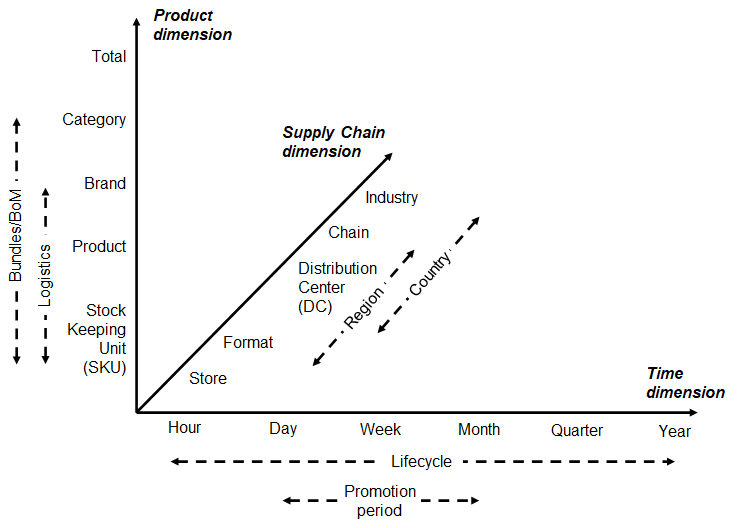
Figure 6: Retail forecasting hierarchy.

Forecasting retail demand happens in a three-dimensional space (Syntetos et al., 2016a): the position in the supply chain hierarchy (store, distribution centre, or chain), the level in the product hierarchy (SKU, brand, category, or total) and the time granularity (day, week, month, quarter, or year). In general, the higher is the position in the supply chain, the lower is the time granularity required, e.g., retailers need daily forecasts for store replenishment and weekly forecasts for DC distribution/logistics activities at the SKU level (Fildes et al., 2019b). Hierarchical forecasting (see §2.10.1) is a promising tool to generate coherent demand forecasts on multiple levels over different dimensions (Oliveira & Ramos, 2019).

Several factors affect retail sales, which often increase substantially during holidays, festivals, and other special events. Price reductions and promotions on own and competitors’ products, as well as weather conditions or pandemics, can also change sales considerably (Huang, Fildes, & Soopramanien, 2019). These factors can coincide to increase complexity yet more, like the weather in the days before public holidays having a major impact on customer demand (Obermair, Holzapfel, & Kuhn, 2023).

Zero sales due to stock-outs or low demand occur very often at the SKU \(\times\) store level, both at weekly and daily granularity. The most appropriate forecasting approaches for intermittent demand are Croston’s method (Croston, 1972), the Syntetos-Boylan approximation (SBA; Aris A Syntetos & Boylan, 2005), and the TSB method (Teunter, Syntetos, & Zied Babai, 2011), all introduced in §2.8.1. These methods were originally proposed to forecast sales of spare parts in automotive and aerospace industries. Intermittent demand forecasting methods are starting to be applied to retail demand (Kolassa, 2016), and the recent M5 competition (Makridakis et al., 2022a, 2022b) will undoubtedly spur further research in this direction.

Univariate forecasting models are the most basic methods retailers may use to forecast demand. They range from simple methods such as simple moving averages or exponential smoothing to ARIMA and ETS models (discussed in §2.3). These are particularly appropriate to forecast demand at higher aggregation levels (Ramos & Oliveira, 2016; Ramos, Santos, & Rebelo, 2015). The main advantage of linear causal methods such as multiple linear regression is to allow the inclusion of external effects discussed above. Simple methods were for a long time found to be superior to more complex and Machine Learning methods (Fildes et al., 2019b), until the M5 competition (Makridakis et al., 2022a, 2022b) showed that ML methods, in particular Gradient Boosting, could indeed outperform them. However, simple methods making due allowance for demand drivers as listed above still have the advantage of being easier to interpret and simpler to care for, so they will continue to have a place in retail forecasting.

To be effective, point estimates should be combined with quantile predictions or prediction intervals for determining safety stock amounts needed for replenishment. However, to the best of our knowledge this is an under-investigated aspect of retail forecasting (Kolassa, 2016; Taylor, 2007), although recent research is starting to address this issue (Hoeltgebaum, Borenstein, Fernandes, & Veiga, 2021).

The online channel accounts for an ever-increasing proportion of retail sales and poses unique challenges to forecasting, beyond the characteristics of brick and mortar (B&M) retail stores. First, there are multiple drivers or predictors of demand that could be leveraged in online retail, but not in B&M:

• Online retailers can fine-tune customer interactions, e.g., through the landing page, product recommendations, or personalised promotions, leveraging the customer’s purchasing, browsing or returns history, current shopping cart contents, or the retailer’s stock position, in order to tailor the message to one specific customer in a way that is impossible in B&M.

• Conversely, product reviews are a type of interaction between the customer and the retailer and other customers which drives future demand.

Next, there are differences in forecast use:

• Forecast use strongly depends on the retailer’s omnichannel strategy (Armstrong, 2017; Melacini, Perotti, Rasini, & Tappia, 2018; Sopadjieva, Dholakia, & Benjamin, 2017): e.g., for “order online, pick up in store” or “ship from store” fulfillment, we need separate but related forecasts for both total online demand and for the demand fulfilled at each separate store.

• Online retailers, especially in fashion, have a much bigger problem with product returns. They may need to forecast how many products are returned overall (e.g., G. Shang et al., 2020), or whether a specific customer will return a specific product.

Finally, there are differences in the forecasting process:

• B&M retailers decouple pricing/promotion decisions and optimisation from the customer interaction, and therefore from forecasting. Online, this is not possible, because the customer has total transparency to competitors’ offerings. Thus, online pricing needs to react much more quickly to competitive pressures – faster than the forecasting cycle.

• Thus, the specific value of predictors is often not known at the time of forecasting: we don’t know yet which customer will log on, so we don’t know yet how many people will see a particular product displayed on their personalised landing page. (Nor do we know today what remaining stock will be displayed.) Thus, changes in drivers need to be “baked into” the forecasting algorithm.

• Feedback loops between forecasting and other processes are thus even more important online: yesterday’s forecasts drive today’s stock position, driving today’s personalised recommendations, driving demand, driving today’s forecasts for tomorrow. Overall, online retail forecasting needs to be more agile and responsive to the latest interactional decisions taken in the web store, and more tightly integrated into the retailer’s interactional tactics and omnichannel strategy.

Systematic research on demand forecasting in an online or omnnichannel context is only starting to appear (e.g. Omar, Klibi, Babai, & Ducq, 2021 who use basket data from online sales to improve omnichannel retail forecasts).

3.2.5 Promotional forecasting⁹⁶

Promotional forecasting is central for retailing (see §3.2.4), but also relevant for many manufacturers, particularly of Fast Moving Consumer Goods (FMCG). In principle, the objective is to forecast sales, as in most business forecasting cases. However, what sets promotional forecasting apart is that we also make use of information about promotional plans, pricing, and sales of complementary and substitute products (Bandyopadhyay, 2009; J.-L. Zhang et al., 2008). Other relevant variables may include store location and format, variables that capture the presentation and location of a product in a store, proxies that characterise the competition, and so on (Andrews, Currim, Leeflang, & Lim, 2008; Van Heerde, Leeflang, & Wittink, 2002).

Three modelling considerations guide us in the choice of models. First, promotional (and associated effects) are proportional. For instance, we do not want to model the increase in sales as an absolute number of units, but instead, as a percentage uplift. We do this to not only make the model applicable to both smaller and larger applications, for example, small and large stores in a retailing chain, but also to gain a clearer insight into the behaviour of our customers. Second, it is common that there are synergy effects. For example, a promotion for a product may be offset by promotions for substitute products. Both these considerations are easily resolved if we use multiplicative regression models. However, instead of working with the multiplicative models, we rely on the logarithmic transformation of the data (see §2.2.1) and proceed to construct the promotional model using the less cumbersome additive formulation (see §2.3.2). Third, the objective of promotional models does not end with providing accurate predictions. We are also interested in the effect of the various predictors: their elasticity. This can in turn provide the users with valuable information about the customers, but also be an input for constructing optimal promotional and pricing strategies (Zhang et al., 2008).

Promotional models have been widely used on brand-level data (for example, Divakar, Ratchford, & Shankar, 2005). However, they are increasingly used on Stock Keeping Unit (SKU) level data (Ma, Fildes, & Huang, 2016; Trapero, Kourentzes, & Fildes, 2015), given advances in modelling techniques. Especially at that level, limited sales history and potentially non-existing examples of past promotions can be a challenge. Trapero et al. (2015) consider this problem and propose using a promotional model that has two parts that are jointly estimated. The first part focuses on the time series dynamics and is modelled locally for each SKU. The second part tackles the promotional part, which pools examples of promotions across SKUs to enable providing reasonable estimates of uplifts even for new SKUs. To ensure the expected heterogeneity in the promotional effects, the model is provided with product group information. Another recent innovation is looking at modelling promotional effects both at the aggregate brand or total sales level, and disaggregate SKU level, relying on temporal aggregation (Kourentzes & Petropoulos, 2016 and §2.10.2). Ma et al. (2016) concern themselves with the intra-and inter-category promotional information. The challenge now is the number of variables to be considered for the promotional model, which they address by using sequential LASSO (see also §2.5.3). Although the aforementioned models have shown very promising results, one has to recognise that in practice promotions are often forecasted using judgmental adjustments, with inconsistent performance (Trapero, Pedregal, Fildes, & Kourentzes, 2013); see also §2.11.2 and §3.7.3.

3.2.6 New product forecasting⁹⁷

Forecasting the demand for a new product accurately has even more consequence with regards to well-being of the companies than that for a product already in the market. However, this task is one of the most difficult tasks managers must deal with simply because of non-availability of past data (Wind, 1981). Much work has been going on for the last five decades in this field. Despite his Herculean attempt to collate the methods reported, Assmus (1984) could not list all even at that time. The methods used before and since could be categorised into three broad approaches (Goodwin et al., 2013a) namely management judgment, consumer judgment and diffusion/formal mathematical models. In general, the hybrid methods combining different approaches have been found to be more useful (Hyndman & Athanasopoulos, 2018; Peres et al., 2010). Most of the attempts in New product Forecasting (NPF) have been about forecasting ‘adoption’ (i.e., enumerating the customers who bought at least one time) rather than ‘sales’, which accounts for repeat purchases also. In general, these attempts dealt with point forecast although there have been some attempts in interval and density forecasting (Meade & Islam, 2001).

Out of the three approaches in NPF, management judgment is the most used approach (Gartner & Thomas, 1993; Kahn, 2002; Lynn, Schnaars, & Skov, 1999) which is reported to have been carried out by either individual managers or group of them. Ozer (2011) and Surowiecki (2005) articulated their contrasting benefits and deficits. The Delphi method (see §2.11.4) has combined the benefits of these two modes of operation (Rowe & Wright, 1999) which has been effective in NPF. Prediction markets in the recent past offered an alternative way to aggregate forecasts from a group of Managers (Meeran, Dyussekeneva, & Goodwin, 2013; Wolfers & Zitzewitz, 2004) and some successful application of prediction markets for NPF have been reported by Plott & Chen (2002) and Karniouchina (2011).

In the second category, customer surveys, among other methods, are used to directly ask the customers the likelihood of them purchasing the product. Such surveys are found to be not very reliable (Morwitz, 1997). An alternative method to avoid implicit bias associated with such surveys in extracting inherent customer preference is conjoint analysis, which makes implicit trade off customers make between features explicit by analysing the customers’ preference for different variants of the product. One analysis technique that attempts to mirror real life experience more is Choice Based Conjoint analysis (CBC) in which customers choose the most preferred product among available choices. Such CBC models used together with the analysis tools such as Logit (McFadden, 1977) have been successful in different NPF applications (Meeran, Jahanbin, Goodwin, & Quariguasi Frota Neto, 2017).

In the third approach, mathematical/formal models known as growth or diffusion curves (see §2.3.18 and §2.3.19) have been used successfully to do NPF (Hu et al., 2019). The non-availability of past data is mitigated by growth curves by capturing the generic pattern of the demand growth of a class of products, which could be defined by a limited number of parameters such as saturation level, inflexion point, etc. For a new product a growth curve can be constituted from well-estimated parameters using analogous products, market intelligence or regression methods. Most extensively used family of growth curves for NPF has started with Bass model (Bass, 1969) that has been extended extensively (Bass, Gordon, Ferguson, & Githens, 2001; Easingwood, Mahajan, & Muller, 1983; Islam & Meade, 2000; Peres et al., 2010; Simon & Sebastian, 1987). A recent applications of NPF focused on consumer electronic goods using analogous products (Goodwin et al., 2013a).

3.2.7 Spare parts forecasting⁹⁸

Spare parts are ubiquitous in modern societies. Their demand arises whenever a component fails or requires replacement. Demand for spare parts is typically intermittent, which means that it can be forecasted using the plethora of parametric and non-parametric methods presented in §2.8. In addition to the intermittence of demand, spare parts have two additional characteristics that make them different from Work-In-Progress and final products, namely: (i) they are generated by maintenance policies and part breakdowns, and (ii) they are subject to obsolescence (Bacchetti & Saccani, 2012; Kennedy, Wayne Patterson, & Fredendall, 2002).

The majority of forecasting methods do not link the demand to the generating factors, which are often related to maintenance activities. The demand for spare parts originates from the replacement of parts in the installed base of machines (i.e., the location and number of products in use), either preventively or upon breakdown of the part (Kim, Dekker, & Heij, 2017). Fortuin (1984) claims that using installed base information to forecast the spare part demand can lead to stock reductions of up to 25%. An overview of the literature that deals with spare parts forecasting with installed base information is given by Van der Auweraer & Boute (2019). Spare parts demand can be driven by the result of maintenance inspections and, in this case, a maintenance-based forecasting model should then be considered to deal with this issue. Such forecasting models include the Delay Time (DT) model analysed in Wang & Syntetos (2011). Using the fitted values of the distribution parameters of a data set related to a hospital pumps, Wang & Syntetos (2011) have shown that when the failure and fault arriving characteristics of the items can be captured, it is recommended to use the DT model to forecast the spare part demand with a higher forecast accuracy. However, when such information is not available, then time series forecasting methods, such as those presented in §2.8.1, are recommended. The maintenance based forecasting is further discussed in §3.2.8.

Given the life cycle of products, spare parts are associated with a risk of obsolescence. Molenaers, Baets, Pintelon, & Waeyenbergh (2012) discussed a case study where 54% of the parts stocked at a large petrochemical company had seen no demand for the last 5 years. Hinton (1999) reported that the US Department of Defence was holding 60% excess of spare parts, with 18% of the parts (with a total value of $1.5 billion) having no demand at all. To take into account the issue of obsolescence in spare parts demand forecasting, Teunter et al. (2011) have proposed the TSB method, which deals with linearly decreasing demand and sudden obsolescence cases. By means of an empirical investigation based on the individual demand histories of 8000 spare parts SKUs from the automotive industry and the Royal Air Force (RAF, UK), Babai, Syntetos, & Teunter (2014) have demonstrated the high forecast accuracy and inventory performance of the TSB method. Other variants of the Croston’s method developed to deal with the risk of obsolescence in forecasting spare parts demand include the Hyperbolic-Exponential Smoothing method proposed by Prestwich, Tarim, Rossi, & Hnich (2014) and the modified Croston’s method developed by Babai, Dallery, Boubaker, & Kalai (2019).

3.2.8 Predictive maintenance⁹⁹

A common classification of industrial maintenance includes three types of maintenance (Montero Jimenez, Schwartz, Vingerhoeds, Grabot, & Salaün, 2020). Corrective maintenance refers to maintenance actions that occur after the failure of a component. Preventive maintenance consists of maintenance actions that are triggered after a scheduled number of units as cycles, kilometers, flights, etc. To schedule the fixed time between two preventive maintenance actions, the Weibull distribution is commonly used (Baptista et al., 2018). The drawbacks of preventive maintenance are related to the replacement of components that still have a remaining useful life; therefore, early interventions imply a waste of resources and too late actions could imply catastrophic failures. Additionally, the preventive intervention itself could be a source of failures too. Finally, predictive maintenance (PdM) complements the previous ones and, essentially, uses predictive tools to determine when actions are necessary (Carvalho et al., 2019). Within this predictive maintenance group, other terms are usually found in the literature as Condition-Based Maintenance and Prognostic and Health Management, (Montero Jimenez et al., 2020).

The role of forecasting in industrial maintenance is of paramount importance. One application is to forecast spare parts (see §3.2.7), whose demands are typically intermittent, usually required to carry out corrective and preventive maintenances (Van der Auweraer & Boute, 2019; Wang & Syntetos, 2011). On the other hand, it is crucial for PdM the forecast of the remaining useful time, which is the useful life left on an asset at a particular time of operation (Si, Wang, Hu, & Zhou, 2011). This work will be focused on the latter, which is usually found under the prognostic stage (Jardine, Lin, & Banjevic, 2006).

The typology of forecasting techniques employed is very ample. Montero Jimenez et al. (2020) classify them in three groups: physics-based models, knowledge-based models, and data-driven models. Physics-based models require high skills on the underlying physics of the application. Knowledge-based models are based on facts or cases collected over the years of operation and maintenance. Although, they are useful for diagnostics and provide explicative results, its performance on prognostics is more limited. In this sense, data-driven models are gaining popularity for the development of computational power, data acquisition, and big data platforms. In this case, data coming from vibration analysis, lubricant analysis, thermography, ultrasound, etc. are usually employed. Here, well-known forecasting models as VARIMAX/GARCH (see also §2.3) are successfully used (Baptista et al., 2018; Cheng, Yu, & Chen, 2012; Garcı́a, Pedregal, & Roberts, 2010; Gomez Munoz, De la Hermosa Gonzalez-Carrato, Trapero Arenas, & Garcia Marquez, 2014). State Space models based on the Kalman Filter are also employed (Pedregal & Carmen Carnero, 2006; Pedregal, Garcı́a, & Roberts, 2009 and §2.3.6). Recently, given the irruption of the Industry 4.0, physical and digital systems are getting more integrated and Machine Learning/Artificial Intelligence are drawing the attention of practitioners and academics alike (Carvalho et al., 2019). In that same reference, it is found that the most frequently used Machine Learning methods in PdM applications were Random Forest, Artificial Neural Networks, Support Vector Machines and K-means.

3.2.9 Reverse logistics¹⁰⁰

As logistics and supply chain operations rely upon accurate demand forecasts (see also §3.2.2), reverse logistics and closed loop supply chain operations rely upon accurate forecasts of returned items. Such items (usually referred as cores) can be anything from reusable shipping or product containers to used laptops, mobile phones or car engines. If some (re)manufacturing activity is involved in supply chains, it is both demand and returned items forecasts that are needed since it is net demand requirements (demand – returns) that drive remanufacturing operations.

Forecasting methods that are known to work well when applied to demand forecasting, such as SES for example (see §2.3.1), do not perform well when applied to time-series of returns because they assume returns to be a process independent of sales. There are some cases when this independence might hold, such as when a recycler receives items sold by various companies and supply chains (Goltsos & Syntetos, 2020). In these cases, simple methods like SES applied on the time series of returns might prove sufficient. Typically though, returns are strongly correlated with past sales and the installed base (number of products with customers). After all, there cannot be a product return if a product has not first been sold. This lagged relationship between sales and returns is key to the effective characterisation of the returns process.

Despite the increasing importance of circular economy and research on closed loop supply chains, returns forecasting has not received sufficient attention in the academic literature (notable contributions in this area include Goh & Varaprasad, 1986; Brito & Laan, 2009; Clottey, Benton, & Srivastava, 2012; Toktay, 2003; Toktay, Wein, & Zenios, 2000). The seminal work by Kelle & Silver (1989) offers a useful framework to forecasting that is based on the degree of available information about the relationship between demand and returns. Product level (PL) information consists of the time series of sales and returns, alongside information on the time each product spends with a customer. The question then is how to derive this time to return distribution. This can be done through managerial experience, by investigating the correlation of the demand and the returns time series, or by serialising and tracking a subset (sample) of items. Past sales can then be used in conjunction with this distribution to create forecasts of returns. Serial number level (SL) information, is more detailed and consists of the time matching of an individual unit item’s issues and returns and thus exactly the time each individual unit, on a serial number basis, spent with the customer. Serialisation allows for a complete characterisation of the time to return distribution. Very importantly, it also enables tracking exactly how many items previously sold remain with customers, providing time series of unreturned past sales. Unreturned past sales can then be extrapolated — along with a time to return distribution — to create forecasts of returns.

Goltsos, Syntetos, & Laan (2019) offered empirical evidence in the area of returns forecasting by analysing a serialised data set from a remanufacturing company in North Wales. They found the Beta probability distribution to best fit times-to-return. Their research suggests that serialisation is something worthwhile pursuing for low volume products, especially if they are expensive. This makes a lot of sense from an investment perspective, since the relevant serial numbers are very few. However, they also provided evidence that such benefits expand in the case of high volume items. Importantly, the benefits of serialisation not only enable the implementation of the more complex SL method, but also the accurate characterisation of the returns process, thus also benefiting the PL method (which has been shown to be very robust).

3.3 Economics and finance

3.3.1 Macroeconomic survey expectations¹⁰¹

Macroeconomic survey expectations allow tests of theories of how agents form their expectations. Expectations play a central role in modern macroeconomic research (Gali, 2008). Survey expectations have been used to test theories of expectations formation for the last 50 years. Initially the Livingston survey data on inflationary expectations was used to test extrapolative or adaptive hypothesis, but the focus soon turned to testing whether expectations are formed rationally (see Turnovsky & Wachter (1972), for an early contribution). According to Muth (1961) p.316, rational expectations is the hypothesis that: ‘expectations, since they are informed predictions of future events, are essentially the same as the predictions of the relevant economic theory.’ This assumes all agents have access to all relevant information. Instead, one can test whether agents make efficient use of the information they possess. This is the notion of forecast efficiency (Mincer & Zarnowitz, 1969), and can be tested by regressing the outturns on a constant and the forecasts of those outturns. Under forecast efficiency, the constant should be zero and the coefficient on the forecasts should be one. When the slope coefficient is not equal to one, the forecast errors will be systematically related to information available at the forecast origin, namely, the forecasts, and cannot be optimal. The exchange between Figlewski & Wachtel (1981, 1983) and Dietrich & Joines (1983) clarifies the role of partial information in testing forecast efficiency (that is, full information is not necessary), and shows that the use of the aggregate or consensus forecast in the individual realisation-forecast regression outlined above will give rise to a slope parameter less than one when forecasters are efficient but possess partial information. Zarnowitz (1985), Keane & Runkle (1990) and Bonham & Cohen (2001) consider pooling across individuals in the realisation-forecast regression, and the role of correlated shocks across individuals.

Recently, researchers considered why forecasters might not possess full-information, stressing informational rigidities: sticky information (see, inter alia, Mankiw & Reis, 2002; Mankiw, Reis, & Wolfers, 2003), and noisy information (see, inter alia, Woodford, 2002; Sims, 2003). Coibion & Gorodnichenko (2012, 2015) test these models using aggregate quantities, such as mean errors and revisions.

Forecaster behaviour can be characterised by the response to new information (see also §2.11.1). Over or under-reaction would constitute inefficiency. Broer & Kohlhas (2018) and Bordalo, Gennaioli, Ma, & Shleifer (2018) find that agents over-react, generating a negative correlation between their forecast revision and error. The forecast is revised by more than is warranted by the new information (over-confidence regarding the value of the new information). Bordalo et al. (2018) explain the over-reaction with a model of ‘diagnostic’ expectations, whereas Fuhrer (2018) finds ‘intrinsic inflation persistence’: individuals under-react to new information, smoothing their responses to news.

The empirical evidence is often equivocal, and might reflect: the vintage of data assumed for the outturns; whether allowance is made for ‘instabilities’ such as alternating over- and under-prediction (Rossi & Sekhposyan, 2016) and the assumption of squared-error loss (see, for example, Patton & Timmermann, 2007; Clements, 2014b).

Research has also focused on the histogram forecasts produced by a number of macro-surveys. Density forecast evaluation techniques such as the probability integral transform¹⁰² have been applied to histogram forecasts, and survey histograms have been compared to benchmark forecasts (see, for example, Bao, Lee, & Saltoglu, 2007; Clements, 2018; Hall & Mitchell, 2009). Research has also considered uncertainty measures based on the histograms Clements (2014a). §2.12.4 and §2.12.5 also discuss the evaluation and reliability of probabilistic forecasts.

Engelberg, Manski, & Williams (2009) and Clements (2009, 2010) considered the consistency between the point predictions and histogram forecasts. Reporting practices such as ‘rounding’ have also been considered (Binder, 2017; Clements, 2011; Manski & Molinari, 2010).

Clements (2019) reviews macroeconomic survey expectations.

3.3.2 Forecasting GDP and inflation¹⁰³

As soon as Bayesian estimation of DSGEs became popular, these models have been employed in forecasting horseraces to predict the key macro variables, for example, Gross Domestic Product (GDP) and inflation, as discussed in Del Negro & Schorfheide (2013). The forecasting performance is evaluated using rolling or recursive (expanded) prediction windows (for a discussion, see Cardani, Paccagnini, & Villa, 2015). DSGEs are usually estimated using revised data, but several studies propose better results estimating the models using real-time data (see, for example, Del Negro & Schorfheide, 2013; Cardani et al., 2019; Kolasa & Rubaszek, 2015b; Wolters, 2015).

The current DSGE model forecasting compares DSGE models to competitors (see §2.3.15 for an introduction to DSGE models). Among them, we can include the Random Walk (the naive model which assumes a stochastic trend), the Bayesian VAR models (Minnesota Prior à la Doan, Litterman, & Sims (1984); and Large Bayesian VAR à la Bańbura, Giannone, & Reichlin (2010)), the Hybrid-Models (the DSGE-VAR à la Del Negro & Schorfheide (2004); and the DSGE-Factor Augmented VAR à la Consolo, Favero, & Paccagnini (2009)), and the institutional forecasts (Greenbook, Survey Professional Forecasts, and the Blue Chip, as illustrated in Edge & Gürkaynak (2010)).

Table 2 summarises the current DSGE forecasting literature mainly for the US and Euro Area and provided by estimating medium-scale models. As general findings, DSGEs can outperform other competitors, with the exception for the Hybrid-Models, in the medium and long-run to forecast GDP and inflation. In particular, Smets & Wouters (2007) was the first empirical evidence of how DSGEs can be competitive with forecasts from Bayesian VARs, convincing researchers and policymakers in adopting DSGEs for prediction evaluations. As discussed in Del Negro & Schorfheide (2013), the accuracy of DSGE forecasts depends on how the model is able to capture low-frequency trends in the data. To explain the macro-finance linkages during the Great Recession, the Smets and Wouters model was also compared to other DSGE specifications including the financial sector. For example, Del Negro & Schorfheide (2013), Kolasa & Rubaszek (2015a), Galvão, Giraitis, Kapetanios, & Petrova (2016), and Cardani et al. (2019) provide forecasting performance for DSGEs with financial frictions. This strand of the literature shows how this feature can improve the baseline Smets and Wouters predictions for the business cycle, in particular during the recent Great Recession.

However, the Hybrid-Models always outperform the DSGEs thanks to the combination of the theory-based model (DSGE) and the statistical representation (VAR or Factor Augmented VAR), as illustrated by Del Negro & Schorfheide (2004) and Consolo et al. (2009).

Moreover, several studies discuss how prediction performance could depend on the parameters’ estimation. Kolasa & Rubaszek (2015b) suggest that updating DSGE model parameters only once a year is enough to have accurate and efficient predictions about the main macro variables.

Table 2: Alternative competitors to DSGE models.

Competitor	Reference
Hybrid Models	US: (Del Negro & Schorfheide, 2004), (Consolo et al., 2009)
Random Walk	US: (Gürkaynak, Kısacıkoğlu, & Rossi, 2013), Euro Area: (Warne et al., 2010), (Smets, Warne, & Wouters, 2014)
Bayesian VAR	US: (Smets & Wouters, 2007), (Gürkaynak et al., 2013), (Wolters, 2015), (Bekiros & Paccagnini, 2014), (S. Bekiros & Paccagnini, 2015), (S. D. Bekiros & Paccagnini, 2015), Euro Area: (Warne et al., 2010)
Time-Varying VAR and Markov-Switching	US: (S. Bekiros et al., 2016), Euro Area: (S. D. Bekiros & Paccagnini, 2016)
Institutional Forecasts	US: (Edge & Gürkaynak, 2010), (Kolasa et al., 2012), (Del Negro & Schorfheide, 2013), (Wolters, 2015)

3.3.3 Forecasting unemployment¹⁰⁴

Unemployment has significant implications at both the micro and macro levels, influencing individual living standards, health and well-being, as well as imposing direct costs on the economy. Given its importance, policy-makers put unemployment at the heart of their economic plans, and as such require accurate forecasts to feed into economic policy decisions. Unemployment is described as a lagging indicator of the economy, with characteristics including business cycles and persistence. Despite this, forecasting the unemployment rate is difficult, because the data are highly non-stationary with abrupt distributional shifts, but persistence within regimes. In this section we focus on methods used to forecast the aggregate unemployment rate.

Unemployment is the outcome of supply and demand for labour, aggregated across all prospective workers, with labour demand derived from demand for goods and services. This implies a highly complex data generating process. Empirical forecasting models tend to simplify this relationship, with two approaches dominating the literature. The first is based on the Phillips (1958) curve capturing a non-linear relationship between nominal wage inflation and the unemployment rate, or the relation between unemployment and output described as Okun’s (1962) Law. The second uses the time-series properties of the data to produce statistical forecasts, such as univariate linear models (for example, ARIMA or unobserved component models; see §2.3.4 and §2.3.6), multivariate linear models (for example, VARMA or CVAR; see §2.3.9), various threshold autoregressive models (see §2.3.13), Markov Switching models (see §2.3.12) and Artificial Neural Networks (see §2.7.8).

The empirical literature is inconclusive as to the ‘best’ forecasting models for unemployment, which varies by country, time period and forecast horizon. There is some evidence that non-linear statistical models tend to outperform within business cycle contractions or expansions, but perform worse across business cycles (see, for example, Montgomery, Zarnowitz, Tsay, & Tiao, 1998; Koop & Potter, 1999; Rothman, 1998), whereas Proietti (2003) finds that linear models characterised by higher persistence perform significantly better. Evidence of non-linearities is found by Peel & Speight (2000), Milas & Rothman (2008) and Johnes (1999), and Gil-Alana (2001) finds evidence of long-memory. Barnichon & Garda (2016) applies a flow approach to unemployment forecasting and finds improvements, as does Smith (2011).

One approach that does yield accurate forecasts is to use a measure of profitability as the explanatory variable, assuming that unemployment will fall when hiring is profitable. D. F. Hendry (2001) proxies profitability (\(\pi\)) by the gap between the real interest rate (reflecting costs) and the real growth rate (reflecting the demand side), such that the unemployment rate rises when the real interest rate exceeds the real growth rate, and vice versa: \[\pi_{t} = \left(R_{L}-\Delta p -\Delta y\right)_{t}\] where \(R_{L}\) is the long-term interest rate, \(\Delta p\) is a measure of inflation and \(\Delta y\) is a measure of output growth. This is then embedded within a dynamic equilibrium correction model, using impulse indicator saturation (IIS: D. F. Hendry et al., 2008b; Johansen & Nielsen, 2009) and step indicator saturation (SIS: Castle et al., 2015a) to capture outliers, breaks and regime shifts, as well as allowing for any non-linearities using Taylor expansions for the regressors. The resulting forecasts perform well over the business cycle relative to alternative statistical models (also see (Hendry, 2015), and (J. L. Castle et al., 2020c)).

Forecasts from models of unemployment could be improved with either better economic theories of aggregate unemployment,¹⁰⁵ or more general empirical models that tackle stochastic trends, breaks, dynamics, non-linearities and interdependence,¹⁰⁶ or better still, both. The COVID-19 pandemic and subsequent lockdown policies highlight just how important forecasts of unemployment are (Castle, Doornik, & Hendry, 2021).

3.3.4 Forecasting productivity¹⁰⁷

The growth of labour productivity, measured by the percent change in output per hours worked, has varied dramatically over the last 260 years. In the UK it ranged from -5.8% at the onset of the 1920 Depression to just over 7% in 1971; see panel A in Figure 7. Productivity growth is very volatile and has undergone large historical shifts with productivity growth averaging around 1% between 1800-1950 followed by an increase in the average annual growth to 3% between 1950-1975. Since the mid-1970’s productivity growth has gradually declined in many developed economies; see panel B of Figure 7. In the decade since 2009, 2% annual productivity growth was an upper bound for most G7 countries.

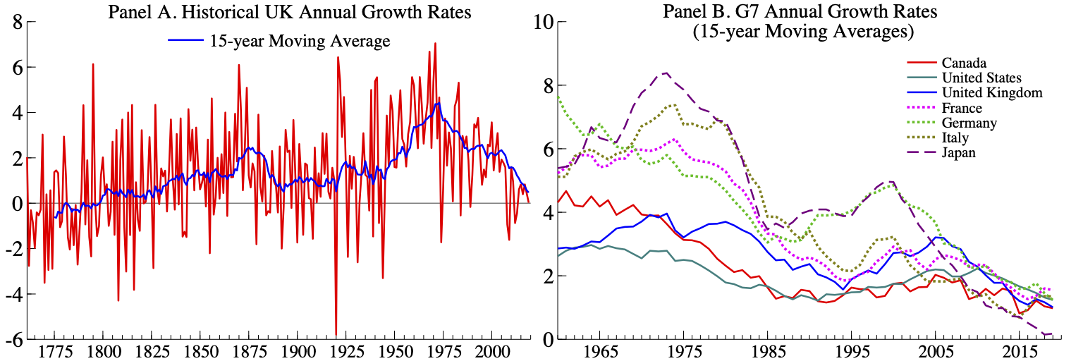
Figure 7: Productivity growth (output per total hours worked). Sources: Bank of England and Penn World Table Version 10.0.

The most common approach for forecasting productivity is to estimate the trend growth in productivity using aggregate data. For example, Gordon (2003) considers three separate approaches for calculating trend labor productivity in the United States based on (i) average historical growth rates outside of the business cycle, (ii) filtering the data using the HP filter (Hodrick & Prescott, 1997), and (iii) filtering the data using the Kalman filter (see Kalman, 1960). The Office for Budget Responsibility (OBR) in the UK and the Congressional Budget Office (CBO) in the US follow similar approaches for generating its forecasts of productivity based on average historical growth rates as well as judgments about factors that may cause productivity to deviate from its historical trend in the short-term.¹⁰⁸ Alternative approaches include forecasting aggregate productivity using disaggregated firm-level data (see Bartelsman, Kurz, & Wolf, 2011; Bartelsman & Wolf, 2014 and §2.10.1) and using time-series models (see Žmuk, Dumičić, & Palić, 2018 and §2.3.4).

In the last few decades there have been several attempts to test for time-varying trends in productivity and to allow for them. However, the focus of these approaches has been primarily on the United States (Hansen, 2001; Roberts, 2001), which saw a sharp rise in productivity growth in the 1990’s that was not mirrored in other countries (Basu, Fernald, Oulton, & Srinivasan, 2003). Test for shifts in productivity growth rates in other advanced economies did not find evidence of a changes in productivity growth until well after the financial crisis in 2007 (Benati, 2007; Glocker & Wegmüller, 2018; Turner & Boulhol, 2011).

A more recent approach by Martinez et al. (2021) allows for a time-varying long-run trend in UK productivity. They show that are able to broadly replicate the OBR’s forecasts using a quasi-transformed autoregressive model with one lag, a constant, and a trend. The estimated long-run trend is just over 2% per year through 2007 Q4 which is consistent with the OBR’s assumptions about the long-run growth rate of productivity (OBR, 2019). However, it is possible to dramatically improve upon OBR’s forecasts in real-time by allowing for the long-term trend forecast to adjust based on more recent historical patterns. By taking a local average of the last four years of growth rates, Martinez et al. (2021) generate productivity forecasts whose RMSE is on average more than 75% smaller than OBR’s forecasts extending five-years-ahead and is 84% smaller at the longest forecast horizon.

3.3.5 Fiscal forecasting for government budget surveillance¹⁰⁹

Recent economic recessions have led to a renewed interest in fiscal forecasting, mainly for deficit and debt surveillance. This was certainly true in the case of the 2008 recession, and looks to become even more important in the current economic crisis brought on by the COVID-19 pandemic. This is particularly important in Europe, where countries are subject to strong fiscal monitoring mechanisms. Two main themes can be detected in the fiscal forecasting literature (Leal, Pérez, Tujula, & Vidal, 2008). First, investigate the properties of forecasts in terms of bias, efficiency and accuracy. Second, check the adequacy of forecasting procedures.

The first topic has its own interest for long, mainly restricted to international institutions (Artis & Marcellino, 2001). Part of the literature, however, argue that fiscal forecasts are politically biased, mainly because there is usually no clear distinction between political targets and rigorous forecasts (Frankel & Schreger, 2013; Strauch, Hallerberg, & Hagen, 2004). In this sense, the availability of forecasts from independent sources is of great value (Jonung & Larch, 2006). But it is not as easy as saying that independent forecasters would improve forecasts due to the absence of political bias, because forecasting accuracy is compromised by complexities of data, country-specific factors, outliers, changes in the definition of fiscal variables, etc. Very often some of these issues are known by the staff of organisations in charge of making the official statistics and forecasts long before the general public, and some information never leaves such institutions. So this insider information is actually a valuable asset to improve forecasting accuracy (Leal et al., 2008).

As for the second issue, namely the accuracy of forecasting methods, the literature can be divided into two parts, one based on macroeconomic models with specific fiscal modules that allows to analyse the effects of fiscal policy on macro variables and vice versa (see Favero & Marcellino (2005) and references therein), and the other based on pure forecasting methods and comparisons among them. This last stream of research basically resembles closely what is seen in other forecasting areas: (i) there is no single method outperforming the rest generally, (ii) judgmental forecasting is especially important due to data problems (see §2.11), and (iii) combination of methods tends to outperform individual ones, see Leal et al. (2008) and §2.6.

Part of the recent literature focused on the generation of very short-term public finance monitoring systems using models that combine annual information with intra-annual fiscal data (Pedregal & Pérez, 2010) by time aggregation techniques (see §2.10.2), often set up in a SS framework (see §2.3.6). The idea is to produce global annual end-of-year forecasts of budgetary variables based on the most frequently available fiscal indicators, so that changes throughout the year in the indicators can be used as early warnings to infer the changes in the annual forecasts and deviations from fiscal targets (Pedregal, Pérez, & Sánchez, 2014).

The level of disaggregation of the indicator variables are established according to the information available and the particular objectives. The simplest options are the accrual National Accounts annual or quarterly fiscal balances running on their cash monthly counterparts. A somewhat more complex version is the previous one with all the variables broken down into revenues and expenditures. Other disaggregation schemes have been applied, namely by region, by administrative level (regional, municipal, social security, etc.), or by items within revenue and/or expenditure (VAT, income taxes, etc. Paredes, Pedregal, & Pérez, 2014; Asimakopoulos, Paredes, & Warmedinger, 2020).

Unfortunately, what is missing is a comprehensive and transparent forecasting system, independent of Member States, capable of producing consistent forecasts over time and across countries. This is certainly a challenge that no one has yet dared to take up.

3.3.6 Interest rate prediction¹¹⁰

The (spot) rate on a (riskless) bond represents the ex-ante return (yield) to maturity which equates its market price to a theoretical valuation. Modelling and predicting default-free, short-term interest rates are crucial tasks in asset pricing and risk management. Indeed, the value of interest rate–sensitive securities depends on the value of the riskless rate. Besides, the short interest rate is a fundamental ingredient in the formulation and transmission of the monetary policy (see, for example, §2.3.15). However, many popular models of the short rate (for instance, continuous time, diffusion models) fail to deliver accurate out-of-sample forecasts. Their poor predictive performance may depend on the fact that the stochastic behaviour of short interest rates may be time-varying (for instance, it may depend on the business cycle and on the stance of monetary policy).

Notably, the presence of nonlinearities in the conditional mean and variance of the short-term yield influences the behaviour of the entire term structure of spot rates implicit in riskless bond prices. For instance, the level of the short-term rate directly affects the slope of the yield curve. More generally, nonlinear rate dynamics imply a nonlinear equilibrium relationship between short and long-term yields. Accordingly, recent research has reported that dynamic econometric models with regime shifts in parameters, such as Markov switching (MS; see §2.3.12) and threshold models (see §2.3.13), are useful at forecasting rates.

The usefulness of MS VAR models with term structure data had been established since Hamilton (1988) and Garcia & Perron (1996): single-state, VARMA models are overwhelmingly rejected in favour of multi-state models. Subsequently, a literature has emerged that has documented that MS models are required to successfully forecast the yield curve. Lanne & Saikkonen (2003) showed that a mixture of autoregressions with two regimes improves the predictions of US T-bill rates. Ang & Bekaert (2002) found support for MS dynamics in the short-term rates for the US, the UK, and Germany. Cai (1994) developed a MS ARCH model to examine volatility persistence, reflecting a concern that it may be inflated by regimes. Gray (1996) generalised this attempt to MS GARCH and reported improvements in pseudo out-of-sample predictions. Further advances in the methods and applications of MS GARCH are in Haas, Mittnik, & Paolella (2004) and Smith (2002). A number of papers have also investigated the presence of regimes in the typical factors (level, slope, and convexity) that characterise the no-arbitrage dynamics of the term structure, showing the predictive benefits of incorporating MS (see, for example, M. Guidolin & Pedio, 2019; Hevia, Gonzalez-Rozada, Sola, & Spagnolo, 2015).

Alternatively, a few studies have tried to capture the time-varying, nonlinear dynamics of interest rates using threshold models. As discussed by Pai & Pedersen (1999), threshold models have an advantage compared to MS ones: the regimes are not determined by an unobserved latent variable, thus fostering interpretability. In most of the applications to interest rates, the regimes are determined by the lagged level of the short rate itself, in a self-exciting fashion. For instance, Pfann, Schotman, & Tschernig (1996) explored nonlinear dynamics of the US short-term interest rate using a (self-exciting) threshold autoregressive model augmented by conditional heteroskedasticity (namely, a TAR-GARCH model) and found strong evidence of the presence of two regimes. More recently, also Gospodinov (2005) used a TAR-GARCH to predict the short-term rate and showed that this model can capture some well-documented features of the data, such as high persistence and conditional heteroskedasticity.

Another advantage of nonlinear models is that they can reproduce the empirical puzzles that plague the expectations hypothesis of interest rates (EH), according to which it is a weighted average of short-term rates to drive longer-term rates (see, for example, Bansal, Tauchen, & Zhou, 2004; Dai, Singleton, & Yang, 2007). For instance, while Bekaert, Hodrick, & Marshall (2001) show single-state VARs cannot generate distributions consistent with the EH, Guidolin & Timmermann (2009) find that the optimal combinations of lagged short and forward rates depend on regimes so that the EH holds only in some states.

As widely documented (see, for instance, M. Guidolin & Thornton, 2018), the predictable component in mean rates is hardly significant. As a result, the random walk remains a hard benchmark to outperform as far as the prediction of the mean is concerned. However, density forecasts reflect all moments and the models that capture the dynamics of higher-order moments tend to perform best. MS models appear at the forefront of a class of non-linear models that produce accurate density predictions (see, for example, Hong, Li, & Zhao, 2004; Maheu & Yang, 2016). Alternatively, Pfann et al. (1996) and more recently Dellaportas, Denison, & Holmes (2007) estimated TAR models to also forecast conditional higher order moments and all report reasonable accuracy.

Finally, a literature has strived to fit rates not only under the physical measure, i.e., in time series, but to predict rates when MS enters the pricing kernel, the fundamental pricing operator. A few papers have assumed that regimes represent a new risk factor (see, for instance, Dai & Singleton, 2003). This literature reports that MS models lead to a range of shapes for nominal and real term structures (see, for instance, Veronesi & Yared, 1999). Often the model specifications that are not rejected by formal tests include regimes (Ang, Bekaert, & Wei, 2008; Bansal & Zhou, 2002).

To conclude, it is worthwhile noting that, while threshold models are more interpretable, MS remain a more popular alternative for the prediction of interest rates. This is mainly due to the fact that statistical inference for threshold regime switching models poses some challenges, because the likelihood function is discontinuous with respect to the threshold parameters.

3.3.7 House price forecasting¹¹¹

The boom and bust in housing markets in the early and mid 2000s and its decisive role in the Great Recession has generated a vast interest in the dynamics of house prices and emphasised the importance of accurately forecasting property price movements during turbulent times. International organisations, central banks and research institutes have become increasingly engaged in monitoring the property price developments across the world.¹¹² At the same time, a substantial empirical literature has developed that deals with predicting future house price movements (for a comprehensive survey see Ghysels, Plazzi, Valkanov, & Torous, 2013). Although this literature concentrates almost entirely on the US (see, for example, Rapach & Strauss, 2009; Bork & Møller, 2015), there are many other countries, such as the UK, where house price forecastability is of prime importance. Similarly to the US, in the UK, housing activities account for a large fraction of GDP and of households’ expenditures; real estate property comprises a significant component of private wealth and mortgage debt constitutes a main liability of households (Office for National Statistics, 2019).

The appropriate forecasting model has to reflect the dynamics of the specific real estate market and take into account its particular characteristics. In the UK, for instance, there is a substantial empirical literature that documents the existence of strong spatial linkages between regional markets, whereby the house price shocks emanating from southern regions of the country, and in particular Greater London, have a tendency to spread out and affect neighbouring regions with a time lag (see, for example, Cook & Thomas, 2003; Antonakakis, Chatziantoniou, Floros, & Gabauer, 2018 inter alia; Holly, Pesaran, & Yamagata, 2010); see also §2.3.10 on forecasting functional data.

Recent evidence also suggests that the relationship between real estate valuations and conditioning macro and financial variables displayed a complex of time-varying patterns over the previous decades (Aizenman & Jinjarak, 2013). Hence, predictive methods that do not allow for time-variation in both predictors and their marginal effects may not be able to capture the complex house price dynamics in the UK (see Yusupova, Pavlidis, & Pavlidis, 2019 for a comparison of forecasting accuracy of a battery of static and dynamic econometric methods).

An important recent trend is to attempt to incorporate information from novel data sources (such as newspaper articles, social media, etc.) in forecasting models as a measure of expectations and perceptions of economic agents (see also §2.9.3). It has been shown that changes in uncertainty about house prices impact on housing investment and real estate construction decisions (Banks, Blundell, Oldfield, & Smith, 2015; Cunningham, 2006; Oh & Yoon, 2020), and thus incorporating a measure of uncertainty in the forecasting model can improve the forecastability of real estate prices. For instance in the UK, the House Price Uncertainty (HPU) index (Yusupova, Pavlidis, Paya, & Peel, 2020), constructed using the methodology outlined in Baker, Bloom, & Davis (2016),¹¹³ was found to be important in predicting property price inflation ahead of the house price collapse of the third quarter of 2008 and during the bust phase (Yusupova et al., 2019). Along with capturing the two recent recessions (in the early 1990s and middle 2000s) this index also reflects the uncertainly related to the EU Referendum, Brexit negotiations and COVID-19 pandemic.

3.3.8 Exchange rate forecasting¹¹⁴

Exchange rates have long fascinated and puzzled researchers in international finance. The reason is that following the seminal paper of Meese & Rogoff (1983), the common wisdom is that macroeconomic models cannot outperform the random walk in exchange rate forecasting (see Rossi, 2013 for a survey). This view is difficult to reconcile with the strong belief that exchange rates are driven by fundamentals, such as relative productivity, external imbalances, terms of trade, fiscal policy or interest rate disparity (Couharde, Delatte, Grekou, Mignon, & Morvillier, 2018; Lee, Milesi-Ferretti, & Ricci, 2013; MacDonald, 1998). These two contradicting assertions by the academic literature is referred to as “exchange rate disconnect puzzle”.

The literature provides several explanations for this puzzle. First, it can be related to the forecast estimation error (see §2.5.2). The studies in which models are estimated with a large panels of data (Engel, Mark, & West, 2008; Ince, 2014; Mark & Sul, 2001), long time series (Lothian & Taylor, 1996) or calibrated (Ca’ Zorzi & Rubaszek, 2020) deliver positive results on exchange rate forecastability. Second, there is ample evidence that the adjustment of exchange rates to equilibrium is non-linear (Curran & Velic, 2019; Taylor & Peel, 2000), which might diminish the out-of-sample performance of macroeconomic models (Kilian & Taylor, 2003; Lopez-Suarez & Rodriguez-Lopez, 2011). Third, few economists argue that the role of macroeconomic fundamentals may be varying over time and this should be accounted for in a forecasting setting (Beckmann & Schussler, 2016; Byrne, Korobilis, & Ribeiro, 2016).

The dominant part of the exchange rate forecasting literature investigates which macroeconomic model performs best out-of-sample. The initial studies explored the role of monetary fundamentals to find that these models deliver inaccurate short-term and not so bad long-term predictions in comparison to the random walk (Mark, 1995; Meese & Rogoff, 1983). In a comprehensive study from mid-2000s, Cheung, Chinn, & Pascual (2005) showed that neither monetary, uncovered interest parity (UIP) nor behavioural equilibrium exchange rate (BEER) model are able to outperform the no-change forecast. A step forward was made by Molodtsova & Papell (2009), who proposed a model combining the UIP and Taylor rule equations and showed that it delivers competitive exchange rate forecasts. This result, however, has not been confirmed by more recent studies (Cheung, Chinn, Pascual, & Zhang, 2019; Engel, Lee, Liu, Liu, & Wu, 2019). In turn, Ca’ Zorzi & Rubaszek (2020) argue that a simple method assuming gradual adjustment of the exchange rate towards the level implied by the Purchasing Power Parity (PPP) performs well over shorter as well as longer horizon. This result is consistent with the results of Ca’ Zorzi et al. (2017) and Eichenbaum, Johannsen, & Rebelo (2017), who showed that exchange rates are predictable within a general equilibrium DSGE framework (see §2.3.15), which encompasses an adjustment of the exchange rate to a PPP equilibrium. Finally, Ca’ Zorzi et al. (2020) discuss how extending the PPP framework for other fundamentals within the BEER framework is not helping in exchange rate forecasting. Overall, at the current juncture it might be claimed that “exchange rate disconnect puzzle” is still puzzling, with some evidence that methods based on PPP and controlling the estimation forecast error can deliver more accurate forecast than the random walk benchmark. A way forward to account for macroeconomic variables in exchange rate forecasting could be to use variable selection methods that allow to control for the estimation error (see §2.5.3).

3.3.9 Financial time series forecasting with range-based volatility models¹¹⁵

The range-based (RB) volatility models is a general term for the models constructed with high and low prices, and most often with their difference i.e., the price range. A short review and classification of such models is contained in §2.3.14. From practical point of view, it is important that low and high prices are almost always available with daily closing prices for financial series. The price range (or its logarithm) is a significantly more efficient estimator of volatility than the estimator based on closing prices (Alizadeh et al., 2002). Similarly the co-range (the covariance based on price ranges) is a significantly more efficient estimator of the covariance of returns than the estimator based on closing prices (Brunetti & Lildholdt, 2002). For these reasons models based on the price range and the co-range better describe variances and covariances of financial returns than the ones based on closing prices.

Forecasts of volatility from simple models like moving average, EWMA, AR, ARMA based on the RB variance estimators are more accurate than the forecasts from the same models based on squared returns of closing prices (Rajvanshi, 2015; Vipul & Jacob, 2007). Forecasts of volatility from the AR model based on the Parkinson estimator are more precise even than the forecasts from the standard GARCH models (see §2.3.11) based on closing prices (H. Li & Hong, 2011).

In plenty of studies it was shown that forecasts of volatility of financial returns from the univariate RB models are more accurate than the forecasts from standard GARCH models based on closing prices (see, for example, Mapa (2003) for the GARCH-PARK-R model; Chou (2005) for the CARR model; Fiszeder (2005) for the GARCH-TR model; Brandt & Jones (2006) for the REGARCH model; Chen et al. (2008) for the TARR model; Lin et al. (2012) for the STARR model; Fiszeder & Perczak (2016) for the GARCH model estimated with low, high and closing prices during crisis periods; Molnár (2016) for the RGARCH model).

The use of daily low and high prices in the multivariate volatility models leads to more accurate forecasts of covariance or covariance matrix of financial returns than the forecasts from the models based on closing prices (see, for example, Chou et al. (2009) for the RB DCC model; Harris & Yilmaz (2010) for the hybrid EWMA model; Fiszeder (2018) for the BEKK-HL model; Piotr Fiszeder & Fałdziński (2019) for the co-range DCC model; Fiszeder et al. (2019) for the DCC-RGARCH model).

The RB models were used in many financial applications. They lead for example to more precise forecasts of value-at-risk measures in comparison to the application of only closing prices (see, for example, Chen, Gerlach, Hwang, & McAleer (2012) for the threshold CAViaR model; Asai & Brugal (2013) for the HVAR model; Fiszeder et al. (2019) for the DCC-RGARCH model; X. Meng & Taylor (2020) for scoring functions). The application of the multivariate RB models provides also the increase in the efficiency of hedging strategies (see, for example, Chou et al. (2009) for the RB DCC model; Harris & Yilmaz (2010) for the hybrid EWMA model; Su & Wu (2014) for the RB-MS-DCC model). Moreover, the RB volatility models have more significant economic value than the return-based ones in the portfolio construction (Chou & Liu (2010) for the RB DCC model; Wu & Liang (2011) for the RB-copula model). Some studies show that based on the forecasts from the volatility models with low and high prices it is possible to construct profitable investment strategies (He, Kwok, & Wan (2010) for the VECM model; Kumar (2015) for the CARRS model).

3.3.10 Copula forecasting with multivariate dependent financial time series¹¹⁶

In this section, we focus on the practical advances on jointly forecasting multivariate financial time series with copulas. In the copula framework (see §2.4.3), because marginal models and copula models are separable, point forecasts are straightforward with marginal models, but dependence information is ignored. A joint probabilistic forecast with copulas involves both estimations of the copula distribution and marginal models.

In financial time series, an emerging interest is to model and forecast the asymmetric dependence. A typical asymmetric dependence phenomenon is that two stock returns exhibit greater correlation during market downturns than market upturns. A. J. Patton (2006) employs the asymmetric dependence between exchange rates with a time-varying copula construction with AR and GARCH margins. A similar study for measuring financial contagion with copulas allows the parameters of the copula to change with the states of the variance to identify shifts in the dependence structure in times of crisis (Rodriguez, 2007).

In stock forecasting, Almeida & Czado (2012) employ a stochastic copula autoregressive model to model DJI and Nasdaq, and the dependence at the time is modelled by a real-valued latent variable, which corresponds to the Fisher transformation of Kendall’s \(\tau\). Li & Kang (2018) use a covariate-dependent copula framework to forecast the time varying dependence that improves both the probabilistic forecasting performance and the forecasting interpretability. Liquidity risk is another focus in finance. Weiß & Supper (2013) forecast three types of liquidity-adjusted intraday Value-at-Risk (L-IVaR) with a vine copula structure. The liquidity-adjusted intraday VaR is based on simulated portfolio values, and the results are compared with the realised portfolio profits and losses.

In macroeconomic forecasting, most existing reduced-form models for multivariate time series produce symmetric forecast densities. Gaussian copulas with skew Student’s-t margins depict asymmetries in the predictive distributions of GDP growth and inflation (Smith & Vahey, 2016). Real-time macroeconomic variables are forecasted with heteroscedastic inversion copulas (Smith & Maneesoonthorn, 2018) that allow for asymmetry in the density forecasts, and both serial and cross-sectional dependence could be captured by the copula function (Rubén Loaiza-Maya & Smith, 2020).

Copulas are also widely used to detect and forecast default correlation, which is a random variable called time-until-default to denote the survival time of each defaultable entity or financial instrument (Li, 2000). Then copulas are used in modelling the dependent defaults (Li, 2000), forecasting credit risk (Bielecki & Rutkowski, 2013), and credit derivatives market forecasting (Schönbucher, 2003). A much large volume of literature is available for this specific area. See the aforementioned references therein. For particular applications in credit default swap (CDS) and default risk forecasting, see Oh & Patton (2018) and Li & He (2019) respectively.

In energy economics, Aloui, Hammoudeh, & Nguyen (2013) employ the time-varying copula approach, where the marginal models are from ARMA(\(p\),\(q\))–GARCH(1,1) to investigate the conditional dependence between the Brent crude oil price and stock markets in the Central and Eastern European transition economies. Bessa, Miranda, Botterud, Zhou, & Wang (2012) propose a time-adaptive quantile-copula where the copula density is estimated with a kernel density forecast method. The method is applied to wind power probabilistic forecasting (see also §3.4.6) and shows its advantages for both system operators and wind power producers. Vine copula models are also used to forecast wind power farms’ uncertainty in power system operation scheduling. Wang, Wang, Liu, Wang, & Hou (2017) shows vine copulas have advantages of providing reliable and sharp forecast intervals, especially in the case with limited observations available.

3.3.11 Financial forecasting with neural networks¹¹⁷

Neural Networks (NNs; see §2.7.8) are capable of successfully modelling non-stationary and non-linear series. This property has made them one of the most popular (if not the most) non-linear specification used by practitioners and academics in Finance. For example, 89% of European banks use NNs to their operations (European Banking Federation, 2019) while 25.4% of the NNs applications in total is in Finance (Wong, Bodnovich, & Selvi, 1995).

The first applications of NNs in Finance and currently the most widespread, is in financial trading. In the mid-80s when computational power became cheaper and more accessible, hedge fund managers started to experiment with NNs in trading. Their initial success led to even more practitioners to apply NNs and nowadays 67% of hedge fund managers use NNs to generate trading ideas (BarclayHedge, 2018). A broad measure of the success of NNs in financial trading is provided by the Eurekahedge AI Hedge Fund Index¹¹⁸ where it is noteworthy the 13.02% annualised return of the selected AI hedge funds over the last 10 years.

In academia, financial trading with NNs is the focus of numerous papers. Notable applications of NNs in trading financial series were provided by Kaastra & Boyd (1996), Tenti (1996), Panda & Narasimhan (2007), Zhang & Ming (2008), and Dunis, Laws, & Sermpinis (2010). The aim of these studies is to forecast the sign or the return of financial trading series and based on these forecasts to generate profitable trading strategies. These studies are closely related to the ones presented in §3.3.13 but the focus is now in profitability. The second major field of applications of NNs in Finance is in derivatives pricing and financial risk management. The growth of the financial industry and the provided financial services have made NNs and other machine learning algorithms a necessity for tasks such as fraud detection, information extraction and credit risk assessment (Buchanan, 2019). In derivatives pricing, NNs try to fill the limitations of the Black-Scholes model and are being used in options pricing and hedging. In academia notable applications of NNs in risk management are provided by Locarek-Junge & Prinzler (1998) and Liu (2005) and in derivatives by Bennell & Sutcliffe (2004) and Psaradellis & Sermpinis (2016).

As discussed before, financial series due to their non-linear nature and their wide applications in practice seems the perfect forecasting data set for researchers that want to test their NN topologies. As a result, there are thousands of forecasting papers in the field of NNs in financial forecasting. However, caution is needed in interpretation of their results. NNs are sensitive to the choice of their hyperparameters. For a simple MLP, a practitioner needs to set (among others) the number and type of inputs, the number of hidden nodes, the momentum, the learning rate, the number of epochs and the batch size. This complexity in NN modelling leads inadvertently to the data snooping bias (see also §2.12.6). In other words, a researcher that experiments long enough with the parameters of a NN topology can have excellent in-sample and out-of-sample results for a series. However, this does not mean that the results of his NN can be generalised. This issue has led the related literature to be stained by studies cannot be extended in different samples.

3.3.12 Forecasting returns to investment style¹¹⁹

Investment style or factor portfolios are constructed from constituent securities on the basis of a variety of a-priori observable characteristics, thought to affect future returns. For example a ‘Momentum’ portfolio might be constructed with positive (‘long’) exposures to stocks with positive trailing 12-month returns, and negative (‘short’) exposure to stocks with negative trailing 12-month returns (for full background and context, see, for example Bernstein, 1995; Haugen, 2010).¹²⁰ Explanations as to why such characteristics seem to predict returns fall in to two main camps: firstly that the returns represent a risk premium, earned by the investor in return for taking on some kind of (undiversifiable) risk, and secondly that such returns are the result of behavioural biases on the part of investors. In practice, both explanations are likely to drive style returns to a greater or lesser extent. Several such strategies have generated reasonably consistent positive risk-adjusted returns over many decades, but as with many financial return series, return volatility is large relative to the mean, and there can be periods of months or even years when returns deviate significantly from their long-run averages. The idea of timing exposure to styles is therefore at least superficially attractive, although the feasibility of doing so is a matter of some debate (Arnott, Beck, Kalesnik, & West, 2016; Asness, 2016; Bender, Sun, Thomas, & Zdorovtsov, 2018). Overconfidence in timing ability has a direct cost in terms of trading frictions and opportunity cost in terms of potential expected returns and diversification forgone.

A number of authors write on the general topic of style timing (recent examples include Hodges, Hogan, Peterson, & Ang, 2017; Dichtl, Drobetz, Lohre, Rother, & Vosskamp, 2019), and several forecasting methodologies have been suggested, falling in to three main camps:

1. Serial Correlation: Perhaps the most promising approach is exploiting serial correlation in style returns. Tarun & Bryan (2019) and Babu, Levine, Ooi, Pedersen, & Stamelos (2020) outline two such approaches and Ehsani & Linnainmaa (2020) explore the relationship between momentum in factor portfolios and momentum in underlying stock returns. As with valuation spreads mentioned below, there is a risk that using momentum signals to time exposure to momentum factor portfolios risks unwittingly compounding exposure. A related strand of research relates (own) factor volatility to future returns, in particular for momentum factors (Barroso, 2015; Daniel & Moskowitz, 2016).

2. Valuation Spreads: Using value signals (aggregated from individual stock value exposures) to time exposure to various fundamental-based strategies is a popular and intuitively appealing approach (Asness, 2016); however evidence of value added from doing so is mixed, and the technique seems to compound risk exposure to value factors.

3. Economic & Financial Conditions: Polk, Haghbin, & Longis (2020) explore how economic and financial conditions affect style returns (an idea that dates back at least to Bernstein (1995) and references therein).

Style returns exhibit distinctly non-normal distributions. On a univariate basis, most styles display returns which are highly negatively skewed and demonstrate significant kurtosis. The long-run low correlation between investment styles is often put forward as a benefit of style-based strategies, but more careful analysis reveals that non-normality extends to the co-movements of investment style returns; factors exhibit significant tail dependence. Christoffersen & Langlois (2013) explores this issue, also giving details of the skew and kurtosis of weekly style returns. These features of the data mean that focusing solely on forecasting the mean may not be sufficient, and building distributional forecasts becomes important for proper risk management. Jondeau (2007) writes extensively on modelling non-gaussian distributions.

3.3.13 Forecasting stock returns¹²¹

Theory and intuition suggest a plethora of potentially relevant predictors of stock returns. Financial statement data (e.g., Chan & Genovese, 2001; Yan & Zheng, 2017) provide a wealth of information, and variables relating to liquidity, price trends, and sentiment, among numerous other concepts, have been used extensively by academics and practitioners alike to predict stock returns. The era of big data further increases the data available for forecasting returns. When forecasting with large numbers of predictors, conventional ordinary least squares (OLS) estimation is highly susceptible to overfitting, which is exacerbated by the substantial noise in stock return data (reflecting the intrinsically large unpredictable component in returns); see §2.7.11.

Over the last decade or so, researchers have explored methods for forecasting returns with large numbers of predictors. Principal component regression extracts the first few principal components (or factors) from the set of predictors; the factors then serve as predictors in a low-dimensional predictive regression, which is estimated via OLS (see §2.7.1). Intuitively, the factors combine the information in the individual predictors to reduce the dimension of the regression, which helps to guard against overfitting. Ludvigson & Ng (2007) find that a few factors extracted from hundreds of macroeconomic and financial variables improve out-of-sample forecasts of the US market return. Kelly & Pruitt (2013) and D. Huang et al. (2015) use partial least squares (Wold, 1966) to construct target-relevant factors from a cross section of valuation ratios and a variety of sentiment measures, respectively, to improve market return forecasts.

Since Bates & Granger (1969), it has been known that combinations of individual forecasts often perform better than the individual forecasts themselves (Timmermann, 2006 and §2.6.1). Rapach, Strauss, & Zhou (2010) show that forecast combination can significantly improve out-of-sample market return forecasts. They first construct return forecasts via individual univariate predictive regressions based on numerous popular predictors from the literature (Goyal & Welch, 2008). They then compute a simple combination forecast by taking the average of the individual forecasts. Rapach et al. (2010) demonstrate that forecast combination exerts a strong shrinkage effect, thereby helping to guard against overfitting.

An emerging literature uses machine-learning techniques to construct forecasts of stock returns based on large sets of predictors. In an investigation of lead-lag relationships among developed equity markets, Rapach, Strauss, & Zhou (2013) appear to be the first to employ machine-learning tools to predict market returns. They use the elastic net (ENet, Zou & Hastie, 2005), a generalisation of the popular least absolute shrinkage and selection operator (LASSO, Tibshirani, 1996). The LASSO and ENet employ penalised regression to guard against overfitting in high-dimensional settings by shrinking the parameter estimates toward zero. Chinco, Clark-Joseph, & Ye (2019) use the LASSO to forecast high-frequency (one-minute-ahead) individual stock returns and report improvements in out-of-sample fit, while Rapach et al. (2019) use the LASSO to improve monthly forecasts of industry returns.

Incorporating insights from Diebold & Shin (2019), Han, He, Rapach, & Zhou (2021) use the LASSO to form combination forecasts of cross-sectional stock returns based on a large number of firm characteristics from the cross-sectional literature (e.g., Harvey, Liu, & Zhu, 2016; Hou, Xue, & Zhang, 2020; McLean & Pontiff, 2016), extending the conventional OLS approach of Haugen & Baker (1996), Lewellen (2015), and Green, Hand, & Zhang (2017). Rapach & Zhou (2020) and Dong, Li, Rapach, & Zhou (n.d.) use the ENet to compute combination forecasts of the market return based on popular predictors from the time-series literature and numerous anomalies from the cross-sectional literature, respectively. Forecasting individual stock returns on the basis of firm characteristics in a panel framework, Freyberger, Neuhierl, & Weber (2020) and Gu, Kelly, & Xiu (2020) employ machine-learning techniques – such as the nonparametric additive LASSO (Huang, Horowitz, & Wei, 2010), random forests (Breiman, 2001), and artificial neural networks – that allow for nonlinear predictive relationships.

3.3.14 Forecasting crashes in stock markets¹²²

Time series data on financial asset returns have special features. Returns themselves are hard to forecast, while it seems that volatility of returns can be predicted. Empirical distributions of asset returns show occasional clusters of large positive and large negative returns. Large negative returns, that is, crashes seem to occur more frequently than large positive returns. Forecasting upcoming increases or decreases in volatility can be achieved by using variants of the Autoregressive Conditional Heteroskedasticity (ARCH) model (Bollerslev, 1986 and §2.3.11; Engle, 1982) or realized volatility models (S. Taylor, 1986). These models take (functions of) past volatility and past returns as volatility predictors, although also other explanatory variables can be incorporated in the regression.

An important challenge that remains is to predict crashes. Sornette (2003) summarises potential causes for crashes and these are computer trading, increased trading in derivatives, illiquidity, trade and budget deficits, and especially, herding behaviour of investors. Yet, forecasting the exact timing of crashes may seem impossible, but on the other hand, it may be possible to forecast the probability that a crash may occur within a foreseeable future. Given the herding behaviour, any model to use for prediction should include some self-exciting behaviour. For that purpose, Aı̈t-Sahalia, Cacho-Diaz, & Laeven (2015) propose mutually exciting jump processes, where jumps can excite new jumps, also across assets or markets (see also Chavez-Demoulin, Davison, & McNeil, 2005). Another successful approach is the Autoregressive Conditional Duration (ACD) model (Engle & Russell, 1997, 1998), which refers to a time series model for durations between (negative) events.

An alternative view on returns’ volatility and the potential occurrence of crashes draws upon the earthquake literature (Ogata, 1978, 1988). The idea is that tensions in and across tectonic plates build up, until an eruption, and after that, tension starts to build up again until the next eruption. By modelling the tension-building-up process using so-called Hawkes processes (Hawkes, 1971, 2018; Hawkes & Oakes, 1974; Ozaki, 1979), one can exploit the similarities between earthquakes and financial crashes (see also §2.8.4). Gresnigt, Kole, & Franses (2015) take Hawkes processes to daily S&P 500 data and show that it is possible to create reliable probability predictions of a crash occurrence within the next five days. Gresnigt et al. (2017a, 2017b) further develop a specification strategy for any type of asset returns, and document that there are spillovers across assets and markets.

Given investor behaviour, past crashes can ignite future crashes. Hawkes processes are particularly useful to describe this feature and can usefully be implemented to predict the probability of nearby crashes. By the way, these processes can also be useful to predict social conflicts, as also there one may discern earthquake-like patterns. Hengel & Franses (2020) document their forecasting power for social conflicts in Africa.

3.4 Energy

3.4.1 Building energy consumption forecasting and optimisation¹²³

In Europe, buildings account for 40% of total energy consumed and 36% of total \(\text{CO}_2\) emissions (Patti et al., 2016). Given that energy consumption of buildings is expected to increase in the coming years, forecasting electricity consumption becomes critical for improving energy management and planning by supporting a large variety of optimisation procedures.

The main challenge in electricity consumption forecasting is that building energy systems are complex in nature, with their behaviour depending on various factors related to the type (e.g., residential, office, entertainment, business, and industrial) and the end-uses (e.g., heating, cooling, hot water, and lighting) of the building, its construction, its occupancy, the occupants’ behaviour and schedule, the efficiency of the installed equipment, and the weather conditions (Zhao & Magoulès, 2012). Special events, holidays, and calendar effects can also affect the behaviour of the systems and further complicate the consumption patterns, especially when forecasting at hourly or daily level (see §2.3.5). As a result, producing accurate forecasts typically requires developing tailored, building-specific methods.

To deal with this task, the literature focuses on three main classes of forecasting methods, namely engineering, statistical, and ML (Mat Daut et al., 2017). Engineering methods, typically utilised through software tools such as DOE-2, EnergyPlus, BLAST, and ESP-r, build on physical models that forecast consumption through detailed equations which account for the particularities of the building (Al-Homoud, 2001; Foucquier, Robert, Suard, Stéphan, & Jay, 2013; Zhao & Magoulès, 2012). Statistical methods usually involve linear regression (see §2.3.2), ARIMA/ARIMAX (see §2.3.4), and exponential smoothing (see §2.3.1) models that forecast consumption using past consumption data or additional explanatory variables, such as weather or occupancy and calendar related information (Deb, Zhang, Yang, Lee, & Shah, 2017). Finally, ML methods (see §2.7.10) typically involve neural networks (see §2.7.8), support vector machines, and grey models that account for multiple non-linear dependencies between the electricity consumed and the factors influencing its value (Ahmad et al., 2014). Till present, the literature has been inconclusive about which class of methods is the most appropriate, with the conclusions drawn being subject to the examined building type, data set used, forecasting horizon considered, and data frequency at which the forecasts are produced (Wei, Li, Peng, Zeng, & Lu, 2019). To mitigate this problem, combinations of methods (see §2.6) and hybrids (see §2.7.13) have been proposed, reporting encouraging results (Mohandes, Zhang, & Mahdiyar, 2019; Zhao & Magoulès, 2012).

Other practical issues refer to data pre-processing. Electricity consumption data is typically collected at high frequencies through smart meters and therefore display noise and missing or extreme values due to monitoring issues (see §2.7.11). As a result, verifying the quality of the input data through diagnostics and data cleansing techniques (see §2.2.3 and §2.2.4), as well as optimising the selected time frames, are important for improving forecasting performance (Bourdeau, Zhai, Nefzaoui, Guo, & Chatellier, 2019). Similarly, it is critical to engineer (see §2.2.5) and select (see §2.5.3) appropriate regressor variables which are of high quality and possible to accurately predict to assist electricity consumption forecasting. Finally, it must be carefully decided whether the bottom-up, the top-down or a combination method (see §2.10.1) will be used for producing reconciled forecasts at both building and end-use level (Kuster, Rezgui, & Mourshed, 2017), being also possibly mixed with temporal aggregation approaches (Spiliotis et al., 2020c but also §2.10.3).

Provided that accurate forecasts are available, effective energy optimisation can take place at a building level or across blocks of buildings (see §3.4.10) to reduce energy cost, improve network stability, and support efforts towards a carbon-free future, by exploiting smart grid, internet of things (IoT), and big data technologies along with recommendation systems (Marinakis et al., 2020).

An example for a typical application in this area is the optimisation of heating, ventilation, and air conditioning (HVAC) systems. The goal is to minimise the energy use of the HVAC system under the constraints of maintaining certain comfort levels in the building (Marinakis, Doukas, Spiliotis, & Papastamatiou, 2017). Though this is predominantly an optimisation exercise, forecasting comes in at different points of the system as input into the optimisation, and many problems in this space involve forecasting as a sub-problem, including energy consumption forecasting, room occupancy forecasting, inside temperature forecasting, (hyper-local) forecasts of outside temperature, and air pressure forecasting for ventilation, among others. For instance, Krüger & Givoni (2004) use a linear regression approach to predict inside temperatures in 3 houses in Brazil, and Ruano, Crispim, Conceiçao, & Lúcio (2006) propose the use of a neural network to predict temperatures in a school building. Madaus, McDermott, Hacker, & Pullen (2020) predict hyper-local extreme heat events, combining global climate models and machine learning models. Jing et al. (2018) predict air pressure to tackle the air balancing problem in ventilation systems, using a support vector machine.

Predicting energy demand on a building/household level from smart meter data is an important research topic not only for energy savings. In the building space, Ahmad, Mourshed, & Rezgui (2017), Touzani, Granderson, & Fernandes (2018), and Zeyu Wang et al. (2018) predict building energy consumption of residential and commercial buildings using decision tree-based algorithms (random forests and gradient boosted trees) and neural networks to improve energy efficiency.

A recent trend in forecasting are global forecasting models, built across sets of time series (Januschowski et al., 2020). (Recurrent) neural networks (Bandara et al., 2020a; Hewamalage et al., 2021) are particularly suitable for this type of processing due to their capabilities to deal with external inputs and cold-start problems. Such capabilities are necessary if there are different regimes in the simulations under which to predict, an example of such a system for HVAC optimisation is presented by Godahewa, Deng, Prouzeau, & Bergmeir (2020).

More generally, many challenges in the space of building energy optimisation are classical examples of so-called “predict then optimise” problems (Demirovic et al., 2019; Elmachtoub & Grigas, 2017). Here, different possible scenario predictions are obtained from different assumptions in the form of input parameters. These input parameters are then optimised to achieve a desired predicted outcome. As both prediction and optimisation are difficult problems, they are usually treated separately (Elmachtoub & Grigas, 2017), though there are now recent works where they are considered together (Demirovic et al., 2019; El Balghiti, Elmachtoub, Grigas, & Tewari, 2019), and this will certainly be an interesting avenue for future research.

3.4.2 Electricity price forecasting¹²⁴

Forecasting electricity prices has various challenges that are highlighted in the detailed review papers by Weron (2014). Even though there are economically well motivated fundamental electricity price models, forecasting models based on evaluating historic price data are the dominating the academic literature. In recent years the focus on probabilistic forecasting grew rapidly, as they are highly relevant for many applications in energy trading and risk management, storage optimisation and predictive maintenance, (Nowotarski & Weron, 2018; Ziel & Steinert, 2018). Electricity price data is highly complex and is influenced by regulation. However, there is electricity trading based on auctions and on continuous trading. Many markets like the US and European markets organise day-ahead auctions for electricity prices, see Figure 8. Thus, we have to predict multivariate time series type data, (Ziel & Weron, 2018). In contrast, intraday markets usually apply continuous trading to manage short term variations due to changes in forecasts of renewable energy and demand, and outages (Kiesel & Paraschiv, 2017).

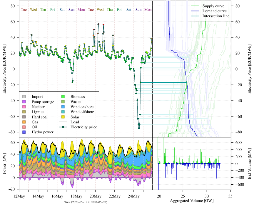
Figure 8: Hourly German day-ahead electricity price data resulting from a two-sided auction (top left) with corresponding 24 sale/supply and purchase/demand curves for 24 May 2020 and highlighted curves for 17:00 (top right), power generation and consumption time series (bottom left), and bid structure of 24 May 2020 17:00 (bottom right).

The key challenge in electricity price forecasting is to address all potential characteristics of the considered market, most notably (some of them visible in Figure 8:

1. (time-varying) autoregressive effects and (in)stationarity,

2. calendar effects (daily, weekly and annual seasonality, holiday effects, clock-change),

3. (time-varying) volatility and higher moment effects,

4. price spikes (positive and negative), and

5. price clustering.

Some of those impacts can be explained by external inputs, that partially have to be predicted in advance:

1. load/demand/consumption (see §3.4.3),

2. power generation, especially from the renewable energy sources (RES) of wind and solar (see §3.4.6 and §3.4.8),

3. relevant fuel prices (especially oil, coal, natural gas; see also §3.4.4),

4. prices of emission allowances (\(CO_2e\) costs),

5. related power market prices (future, balancing and neighboring markets),

6. availabilities of power plants and interconnectors,

7. import/export flow related data, and

8. weather effects (e.g. temperature due to cooling and heating and combined heat and power (CHP) effects; see also §3.5.2).

Note that other weather effects might be relevant as well, but should be covered from the fundamental point of view by the listed external inputs. Obvious examples are wind speed for the wind power prediction, cloud cover for the solar power production and illumination effects in the electricity consumption.

Many of those external effects may be explained by standard economic theory from fundamental electricity price models (Cludius, Hermann, Matthes, & Graichen, 2014; Kulakov & Ziel, 2021). Even the simple supply stack model (merit order model), see Figure 9, explains many features and should be kept in mind when designing an appropriate electricity price forecasting model.

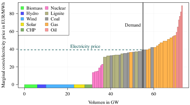
Figure 9: Illustrative example of a supply stack model with inelastic demand for different power plant types, roughly covering the situation in Germany 2020.

In recent years, statistical and machine learning methods gained a lot of attraction in day-ahead electricity price forecasting. Even though the majority of effects is linear there are specific non-linear dependencies that can be explored by using non-linear models, especially neural networks (Dudek, 2016; Lago, De Ridder, & De Schutter, 2018; Marcjasz, Uniejewski, & Weron, 2019; Ugurlu, Oksuz, & Tas, 2018). Of course this comes along with higher computational costs compared to linear models. Fezzi & Mosetti (2020) illustrate that even simple linear models can give highly accurate forecasts, if correctly calibrated. However, there seems to be consensus that forecast combination is appropriate, particularly for models that have different structures or different calibration window length (Gaillard, Goude, & Nedellec, 2016; Hubicka, Marcjasz, & Weron, 2018; Mirakyan, Meyer-Renschhausen, & Koch, 2017).

Another increasing stream of electricity price forecasting models do not focus on the electricity price itself, but the bid/sale/sell/supply and ask/sell/purchase/demand curves of the underlying auctions (see Figure 8, but also Ziel & Steinert, 2016; Kulakov, 2020; Mestre, Portela, San Roque, & Alonso, 2020; Shah & Lisi, 2020). This sophisticated forecasting problem allows more insights for trading applications and the capturing of price clusters.

In forecasting intraday markets the literature just started to grow quickly. As the aforementioned market characteristics get less distinct if information from day-ahead markets is taken into account appropriately. However, intraday prices are usually more volatile and exhibit more stronger price spikes. Thus, probabilistic forecasting is even more relevant (Janke & Steinke, 2019; Narajewski & Ziel, 2020b). Recent studies showed that European markets are close to weak-form efficiency. Thus naive point forecasting benchmarks perform remarkably well (Marcjasz, Uniejewski, & Weron, 2020; Narajewski & Ziel, 2020a; Oksuz & Ugurlu, 2019).

As pointed out above, predicting price spikes is particularly important in practice, due to the high impact in decision making problems which occur usually in extreme situations, see Figure 9. Very high electricity prices are usually observed in connection to high demand and low renewable energy generation, sometimes together with sudden power plant failures. In contrast, negative price spikes occur in oversupply situation, when there is low demand but high penetration from wind and solar power. The presence of spikes is explored in two main streams in literature: spike forecasting and prediction of prices under normal regime through robust estimators.

Within the first set of papers, spikes are often modelled as one regime of non-linear models for time series. This approach is followed by Mount, Ning, & Cai (2006) focusing on regime-switching models with parameters driven by time-varying variables and by Becker, Hurn, & Pavlov (2008) who adopt Markov switching models for spikes prediction. Christensen, Hurn, & Lindsay (2009, 2012) suggest treating and forecasting price spikes through Poisson autoregressive and discrete-time processes, respectively. Herrera & González (2014) use a Hawkes model combined with extreme events theory. Interregional links among different electricity markets are used by Clements, Herrera, & Hurn (2015) and Manner, Türk, & Eichler (2016) to forecast electricity price spikes. A new procedure for the simulation of electricity spikes has been recently proposed by Muniain & Ziel (2020) utilising bivariate jump components in a mean reverting jump diffusion model in the residuals.

The second stream of literature includes papers developing outlier detection methods or robust estimators to improve the forecasting performance of the models. Martı́nez–Álvarez, Troncoso, Riquelme, & Aguilar–Ruiz (2011) tackle the issue of outlier detection and prediction defining “motifs”, that is patches of units preceding observations marked as anomalous in a training set. Janczura, Trück, Weron, & Wolff (2013) focus on the detection and treatment of outliers in electricity prices. A very similar approach, based on seasonal autoregressive models and outlier filtering, is followed by Afanasyev & Fedorova (2019). Grossi & Nan (2019) introduced a procedure for the robust statistical prediction of electricity prices. The econometric framework is represented by the robust estimation of non-linear SETAR processes. A similar approach has been followed by Jianzhou Wang et al. (2020) using an outlier-robust machine learning algorithm.

3.4.3 Load forecasting¹²⁵

Load forecasting forms the basis where power system operation and planning builds upon. Based on the time horizon of the forecasts, load forecasting can be classified into very short-term (VSTLF), that refers to horizon from several minutes ahead up to 1 hour, short-term (STLF), that spans from 1 hour to 168 hours ahead, medium-term (MTLF), that spans from 168 hours to 1 year ahead and finally, and long-term (LTLF) that concerns predictions from 1 year to several years ahead. In VSTLF and STLF applications, the focus is on the sub-hourly or hourly load. In MTLF and LTLF, the variables of interest can be either monthly electricity peak load and total demand for energy.

Inputs differ in the various horizons. In VSTLF and STLF, apart from meteorological data, day type identification codes are used. In LTLF, macroeconomic data are used since total demand of energy is influenced by the long-term modifications of the social and economic environments. Among the horizons, special attention is placed at STLF. This is reflected by the research momentum that have been placed in the load forecasting related literature by other researchers (Hong & Fan, 2016). Processes like unit commitment and optimal power flow rely on STLF (Bo & Li, 2012; Saksornchai, Wei-Jen Lee, Methaprayoon, Liao, & Ross, 2005). Additionally, since competitive energy markets continually evolve, STLF becomes vital for new market entities such as retailers, aggregators, and prosumers for applications such as strategic bidding, portfolio optimisation, and tariff design (Ahmad, Javaid, Mateen, Awais, & Khan, 2019; Danti & Magnani, 2017).

The models that can be found in the load forecasting related literature can in general categorised into three types: time-series, machine learning, and hybrid. Time-series models historically precede the others. Typical examples of this family are ARMA, ARIMA, and others (see also §2.3.4). In the machine learning models, the structure is usually determined via the training process. NNs are commonly used. Once a NN is sufficiently trained, it can provide forecasts for all types of forecasting horizons (Hippert, Pedreira, & Souza, 2001). The third category of models refers to the integration of two or more individual forecasting approaches (see also see §2.7.13). For instance, a NN can be combined with time series methods, with unsupervised machine learning algorithms, data transformation, and with meta-heuristics algorithms (Bozkurt, Biricik, & Tayşi, 2017; El-Hendawi & Wang, 2020; López, Zhong, & Zheng, 2017; H. Lu et al., 2019).

Hybrid systems has been tested on validation data (through forecasting competitions), power system aggregated load, and application oriented tasks. Ma (2021) proposed an ensemble method based on a combination of various single forecasters on GEFCom2012 forecasting competition data that outperformed benchmark forecasters such as Theta method, NN, ARIMA, and others (see §2.12.7 for further discussions on forecasting competitions). For aggregated load cases, researchers focus on different countries and energy markets. J. Zhang et al. (2018) combined empirical mode decomposition (EMD), ARIMA, and wavelet neural networks (WNN) optimised by the fruit fly algorithm on Australian Market data and New York City data. Their approach was to separate the linear and nonlinear components from original electricity load; ARIMA is used for linear part while the WNN for the non-linear one.

Sideratos, Ikonomopoulos, & Hatziargyriou (2020) proposed that a radial basis network that performs the initial forecasting could serve as input to a convolutional neural network that performs the final forecasting. The proposed model led to lower error compared to the persistence model, NN, and SVM. Semero, Zhang, & Zheng (2020) focused on the energy management of a microgrid located in China using EMD to decompose the load, adaptive neuro-fuzzy inference system (ANFIS) for forecasting and particle swarm intelligence (PSO) to optimize ANFIS parameters. The results show that the proposed approach yielded superior performance over four other methods. Faraji, Ketabi, Hashemi-Dezaki, Shafie-Khah, & Catalão (2020) proposed a hybrid system for the scheduling of a prosumer microgrid in Iran. Various machine learning algorithms provided load and weather forecasts. Through an optimisation routine, the best individual forecast is selected. The hybrid system displayed better accuracy from the sole application of the individual forecasters.

3.4.4 Crude oil price forecasting¹²⁶

Crude oil, one of the leading energy resources, has contributed to over one-third of the world’s energy consumption (Alvarez-Ramirez, Soriano, Cisneros, & Suarez, 2003). The fluctuations of the crude oil price have a significant impact on industries, governments as well as individuals, with substantial up-and-downs of the crude oil price bringing dramatic uncertainty for the economic and political development (Cunado & De Gracia, 2005; Kaboudan, 2001). Thus, it is critical to develop reliable methods to accurately forecast crude oil price movement, so as to guard against the crude oil market extreme risks and improve macroeconomic policy responses. However, the crude oil price movement suffers from complex features such as nonlinearity, irregularities, dynamics and high volatility (Alquist, Kilian, & Vigfusson, 2013; Herrera, Hu, & Pastor, 2018 and also §2.3.11; Kang, Kang, & Yoon, 2009), making the crude oil price forecasting still one of the most challenging forecasting problems.

Some prior studies have suggested that the crude oil price movement is inherently unpredictable, and it would be pointless and futile to attempt to forecast future prices, see Miao, Ramchander, Wang, & Yang (2017) for a detailed summary. These agnostics consider the naive no-change forecast as the best available forecast value of future prices. In recent years, however, numerous studies result in forecasts that are more accurate than naive no-change forecasts, making the forecasting activities of crude oil prices promising (Alquist et al., 2013; Baumeister et al., 2015).

Extensive research on crude oil price forecasting has focused predominantly on the econometric models, such as VAR, ARCH-type, ARIMA, and Markov models (see, for example, Mirmirani & Li, 2004; Agnolucci, 2009; Mohammadi & Su, 2010; Silva, Legey, & Silva, 2010 and §2.3). In the forecasting literature, unit root tests (see §2.3.4) are commonly applied to examine the stationarity of crude oil prices prior to econometric modelling (Rahman & Serletis, 2012; Serletis & Rangel-Ruiz, 2004; Silvapulle & Moosa, 1999). It is well-documented that crude oil prices are driven by a large set of external components, which are themselves hard to predict, including supply and demand forces, stock market activities, oil-related events (e.g., war, weather conditions), political factors, etc. In this context, researchers have frequently considered structural models (see §2.3.9), which relate the oil price movements to a set of economic factors. With so many econometric models, is there an optimal one? Recently, Albuquerquemello, Medeiros, Nóbrega Besarria, & Maia (2018) proposed a SETAR model, allowing for predictive regimes changing after a detected threshold, and achieved performance improvements over six widely used econometric models. Despite their high computational efficiency, the econometric models are generally limited in the ability to nonlinear time series modelling.

On the other hand, artificial intelligence and machine learning techniques, such as belief networks, support vector machines (SVMs), recurrent neural networks (RNNs), and extreme gradient boosting (XGBoost), provided powerful solutions to recognise the nonlinear and irregular patterns of the crude oil price movement with high automation (see, for example, Abramson & Finizza, 1991; Gumus & Kiran, 2017; Mingming & Jinliang, 2012; Xie, Yu, Xu, & Wang, 2006). However, challenges also exist in these techniques, such as computational cost and overfitting. In addition, a large number of studies have increasingly focused on the hybrid forecasting models (see also §2.7.13) based on econometrics models and machine learning techniques (Baumeister & Kilian, 2015; Chiroma, Abdulkareem, & Herawan, 2015; He, Yu, & Lai, 2012; Jammazi & Aloui, 2012), achieving improved performance. Notably, the vast majority of the literature has focused primarily on the deterministic prediction, with much less attention paid to the probabilistic prediction and uncertainty analysis. However, the high volatility of crude oil prices makes probabilistic prediction more crucial to reduce the risk in decision-making (Abramson & Finizza, 1995; Sun, Sun, Wang, & Wei, 2018).

3.4.5 Forecasting renewable energy technologies¹²⁷

The widespread adoption of renewable energy technologies, RETs, plays a driving role in the transition to low-carbon energy systems, a key challenge to face climate change and energy security problems. Forecasting the diffusion of RETs is critical for planning a suitable energy agenda and setting achievable targets in terms of electricity generation, although the available time series are often very short and pose difficulties in modelling. According to K. U. Rao & Kishore (2010), renewables’ typical characteristics such as low load factor, need for energy storage, small size, high upfront costs create a competitive disadvantage, while Nigel Meade & Islam (2015b) suggested that renewable technologies are different from other industrial technological innovations because, in the absence of focused support, they are not convenient from a financial point of view. In this sense, policy measures and incentive mechanisms, such as feed-in tariffs, have been used to stimulate the market. As highlighted in C.-Y. Lee & Huh (2017b), forecasting RETs requires to capture different socio-economic aspects, such as policy choices by governments, carbon emissions, macroeconomic factors, economic and financial development of a country, competitive strength of traditional energy technologies.

The complex and uncertain environment concerning RETs deployment has been faced in literature in several ways, in order to account for various determinants of the transition process. A first stream of research employed a bottom-up approach, where forecasts at a lower level are aggregated to higher levels within the forecasting hierarchy. For instance Park, Yun, Yun, Lee, & Choi (2016) realised a bottom-up analysis to study the optimum renewable energy portfolio, while C.-Y. Lee & Huh (2017a) performed a three-step forecasting analysis, to reflect the specificities of renewable sources, by using different forecasting methods for each of the sources considered. A similar bottom-up perspective was adopted in Zhang, Bauer, Yin, & Xie (2020), by conducting a multi-region study, to understand how multi-level learning may affect RETs dynamics, with the regionalised model of investment and technological development, a general equilibrium model linking a macro-economic growth with a bottom-up engineering-based energy system model.

The relative newness of RETs has posed the challenge of forecasting with a limited amount of data: in this perspective, several contributions applied the ‘Grey System’ theory, a popular methodology for dealing with systems with partially unknown parameters (Kayacan, Ulutas, & Kaynak, 2010). Grey prediction models for RETs forecasting were proposed in Tsai et al. (2017), S.-L. Lu (2019), Wu, Ma, Zeng, Wang, & Cai (2019), Moonchai & Chutsagulprom (2020), and Liu & Wu (2021).

Other studies developed forecasting procedures based on growth curves and innovation diffusion models (see §2.3.18, §2.3.19, and §2.3.20): from the seminal work by Marchetti & Nakicenovic (1979), contributions on the diffusion of RETs were proposed by Guidolin & Mortarino (2010), Dalla Valle & Furlan (2011), Nigel Meade & Islam (2015b), C.-Y. Lee & Huh (2017b), and Bunea, Della Posta, Guidolin, & Manfredi (2020). Forecasting the diffusion of renewable energy technologies was also considered within a competitive environment in Huh & Lee (2014), Guidolin & Guseo (2016), Furlan & Mortarino (2018), and Guidolin & Alpcan (2019).

3.4.6 Wind power forecasting¹²⁸

Wind energy is a leading source of renewable energy, meeting 4.8% of global electricity demand in 2018, more than twice that of solar energy (IEA, Paris, 2020). Kinetic energy in the wind is converted into electrical energy by wind turbines according to a characteristic ‘power curve’. Power production is proportion to the cube of the wind speed at low-to-moderate speeds, and above this is constant at the turbine’s rated power. At very high or low wind speeds no power is generated. Furthermore, the power curve is influenced by additional factors including air density, icing, and degradation of the turbine’s blades.

Forecasts of wind energy production are required from minutes to days-ahead to inform the operation of wind farms, participation in energy markets and power systems operations. However, the limited predictability of the weather (see also §3.5.2) and the complexity of the power curve make this challenging. For this reason, probabilistic forecasts are increasing used in practice (Bessa et al., 2017). Their value for energy trading is clear (Pinson, Chevallier, & Kariniotakis, 2007), but quantifying value for power system operation is extremely complex. Wind power forecasting may be considered a mature technology as many competing commercial offerings exist, but research and development efforts to produce novel and enhanced products is ongoing (see also §3.4.5).

Short-term forecasts (hours to days ahead) of wind power production are generally produced by combining numerical weather predictions (NWP) with a model of the wind turbine, farm or even regional power curve, depending on the objective. The power curve may be modelled using physical information, e.g. provided by the turbine manufacturer, in which case it is also necessary to post-process NWP wind speeds to match the same height-above-ground as the turbine’s rotor. More accurate forecasts can be produced by learning the NWP-to-energy relationship from historic data when it is available. State-of-the-art methods for producing wind power forecasts leverage large quantities of NWP data to produce a single forecast (Andrade, Filipe, Reis, & Bessa, 2017) and detailed information about the target wind farm (C. Gilbert et al., 2020a). A number of practical aspects may also need to be considered by users, such as maintenance outages and requirements to reduce output for other reasons, such as noise control or electricity network issues.

Very short-term forecast (minutes to a few hours ahead) are also of value, and on these time scales recent observations are the most significant input to forecasting models and more relevant than NWP. Classical time series methods perform well (see §2.3), and those which are able to capture spatial dependency between multiple wind farms are state-of-the-art, notably vector autoregressive models and variants (Cavalcante, Bessa, Reis, & Browell, 2016; Messner & Pinson, 2018). Care must be taken when implementing these models as wind power time series are bounded by zero and the wind farm’s rated power meaning that errors may not be assumed to be normally distributed. The use of transformations is recommended (see also §2.2.1), though the choice of transformation depends on the nature of individual time series (P. Pinson, 2012).

Wind power forecasting is reviewed in detail in Zhang, Wang, & Wang (2014), Giebel & Kariniotakis (2017), Hong et al. (2020) and research is ongoing in a range of directions including: improving accuracy and reducing uncertainty in short-term forecasting, extending forecast horizons to weeks and months ahead, and improving very short-term forecast with remote sensing and data sharing (Sweeney, Bessa, Browell, & Pinson, 2019 and §3.4.10).

3.4.7 Wave forecasting¹²⁹

Ocean waves are primarily generated by persistent winds in one direction. The energy thus propagated by the wind is referred to as wave energy flux and follows a linear function of wave height squared and wave period. Wave height is typically measured as significant wave height, the average height of the highest third of the waves. The mean wave period, typically measured in seconds, is the average time between the arrival of consecutive crests, whereas the peak wave period is the wave period at which the highest energy occurs at a specific point.

The benefit of wave energy is that it requires significantly less reserve compared to those from wind (see §3.4.6) and solar (see §3.4.8) renewable energy sources (Hong, Pinson, et al., 2016). For example, the forecast error at one hour ahead for the simulated wave farms is typically in the range of 5–7%, while the forecast errors for solar and wind are 17 and 22% respectively (Reikard, Pinson, & Bidlot, 2011). Solar power is dominated by diurnal and annual cycles but also exhibits nonlinear variability due to factors such as cloud cover, temperature and precipitation. Wind power is dominated by large ramp events such as irregular transitions between states of high and low power. Wave energy exhibits annual cycles and is generally smoother although there are still some large transitions, particularly during the winter months. In the first few hours of forecasting wave energy, time series models are known to be more accurate than numerical wave prediction. Beyond these forecast horizons, numerical wave prediction models such as SWAN (Simulating WAves Nearshore, Booij, Ris, & Holthuijsen, 1999) and WAVEWATCH III (Tolman, 2008) are widely used. As there is as yet no consensus on the most efficient model for harnessing wave energy, potential wave energy is primarily measured with energy flux, but the wave energy harnessed typically follows non-linear functions of wave height and wave period in the observations of the six different types of wave energy converters (Reikard, Robertson, Buckham, Bidlot, & Hiles, 2015).

To model the dependencies of wind speed, wave height, wave period and their lags, Reikard et al. (2011) uses linear regressions, which were then converted to forecasts of energy flux. P. Pinson et al. (2012) uses Reikard et al. (2011)’s regression model and log-normal distribution assumptions to produce probabilistic forecasts. López-Ruiz, Bergillos, & Ortega-Sánchez (2016) model the temporal dependencies of significant wave heights, peak wave periods and mean wave direction using a vector autoregressive model, and used them to produce medium to long term wave energy forecasts. Jeon & Taylor (2016) model the temporal dependencies of significant wave heights and peak wave periods using a bivariate VARMA-GARCH (see also §2.3.11) to convert the two probabilistic forecasts into a probabilistic forecast of wave energy flux, finding this approach worked better than either univariate modelling of wave energy flux or bivariate modelling of wave energy flux and wind speed. Taylor & Jeon (2018) produce probabilistic forecasts for wave heights using a bivariate VARMA-GARCH model of wave heights and wind speeds, and using forecasts so as to optimise decision making for scheduling offshore wind farm maintenance vessels dispatched under stochastic uncertainty. On the same subject, C. Gilbert et al. (2020b) use statistical post-processing of numerical wave predictions to produce probabilistic forecasts of wave heights, wave periods and wave direction and a logistic regression to determine the regime of the variables. They further applied the Gaussian copula to model temporal dependency but this did not improve their probabilistic forecasts of wave heights and periods.

3.4.8 Solar power forecasting¹³⁰

Over the past few years, a number of forecasting techniques for photovoltaic (PV) power systems has been developed and presented in the literature. In general, the quantitative comparison among different forecast techniques is challenging, as the factors influencing the performance are numerous: the historical data, the weather forecast, the temporal horizon and resolution, and the installation conditions. A recent review by Sobri, Koohi-Kamali, & Rahim (2018) presents a comparative analysis of previous works, also including statistical errors. However, since the conditions and metrics used in each work were different, the comparison is not very meaningful. Dolara, Grimaccia, Leva, Mussetta, & Ogliari (2018) present relevant evaluation metrics for PV forecasting accuracy, while Leva, Mussetta, & Ogliari (2019) compare their effectiveness and immediate comprehension. In term of forecast horizon for PV power systems, intraday (Nespoli et al., 2019) and the 24 hours of the next day (Mellit et al., 2020) are considered the most important.

Nespoli et al. (2019) compared two of the most widely used and effective methods for the forecasting of the PV production: a method based on Multi-Layer Perceptron (MLP) and a hybrid method using artificial neural network combined with clear sky solar radiation (see also §2.7.8 and §2.7.13). In the second case, the simulations are based on a feed-forward neural network (FFNN) but, among the inputs, the irradiation in clear sky conditions is provided. This method is called Physical Hybrid Artificial Neural Network (PHANN) and is graphically depicted in Figure 10 (Dolara, Grimaccia, Leva, Mussetta, & Ogliari, 2015). PHANN method demonstrates better performance than classical NN methods. Figure 11 shows a comparison between the measured and forecasted hourly output power of the PV plant for both sunny and cloudy days. The PHANN method shows good forecasting performance, especially for sunny days.

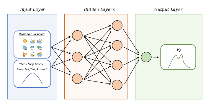
Figure 10: Physical Hybrid Artificial Neural Network (PHANN) for PV power forecasting.

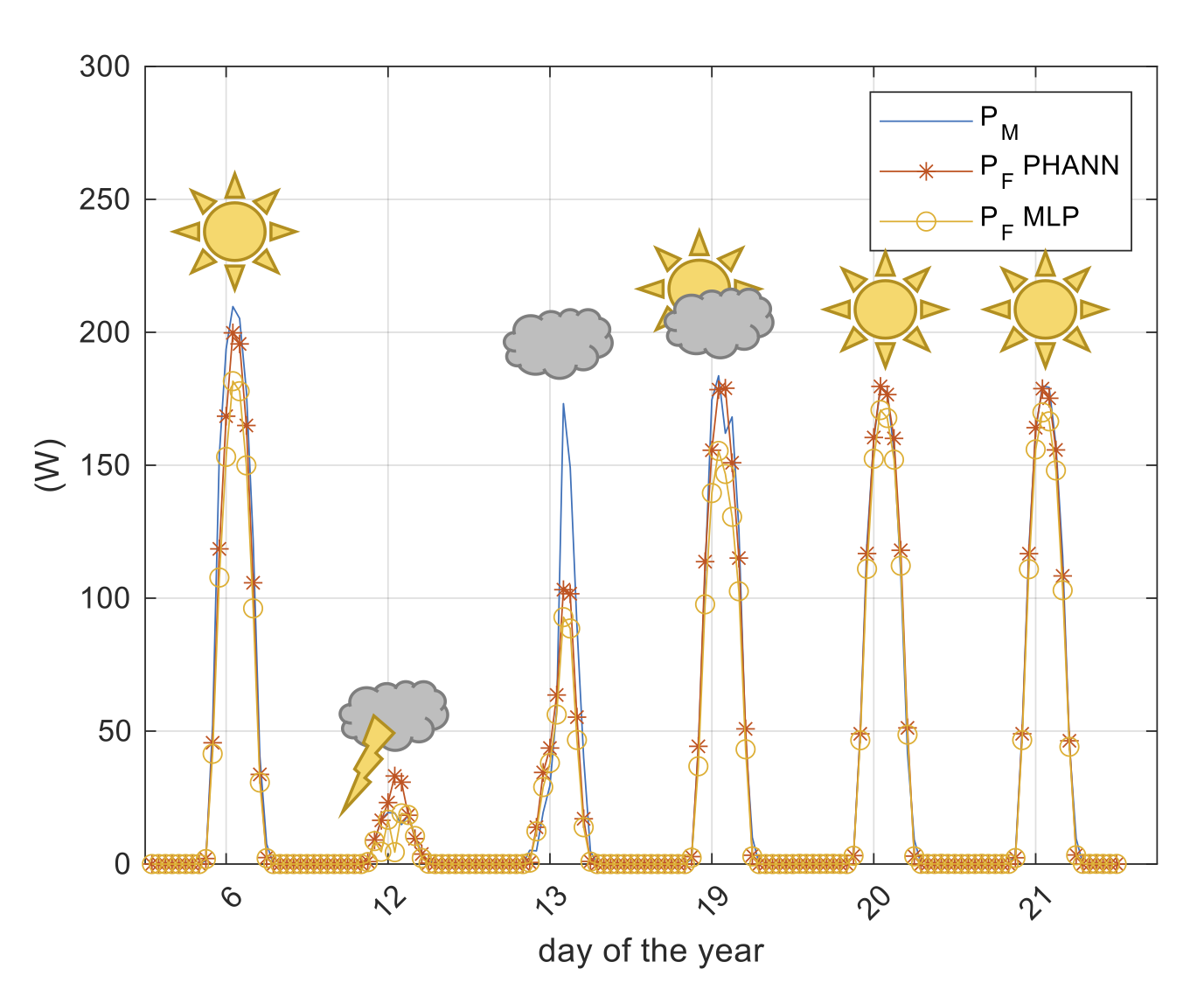
Figure 11: Measured versus forecasted output power by MLP and PHANN methods.

Ogliari, Dolara, Manzolini, & Leva (2017) compared the PV output power day-ahead forecasts performed by deterministic (based on three and five parameters electric equivalent circuit) and stochastic hybrid (based on artificial neural network models) methods aiming to find the best performance conditions. In general, there is no significant difference between the two deterministic models, with the three-parameter approach being slightly more accurate. Figure 12 shows the daily value of normalised mean absolute error (NMAE%) for 216 days evaluated by using PHANN and three parameters electric circuit. The PHANN hybrid method achieves the best forecasting results, and only a few days of training can provide accurate forecasts.

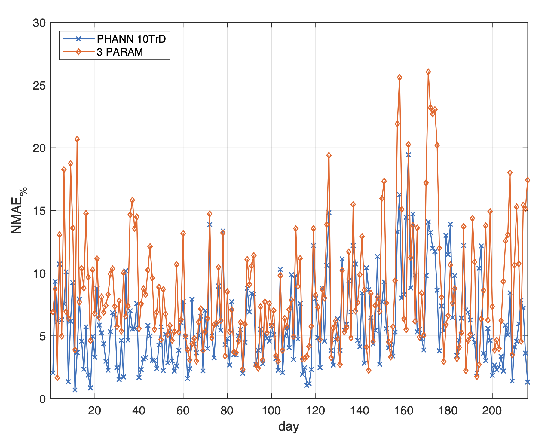
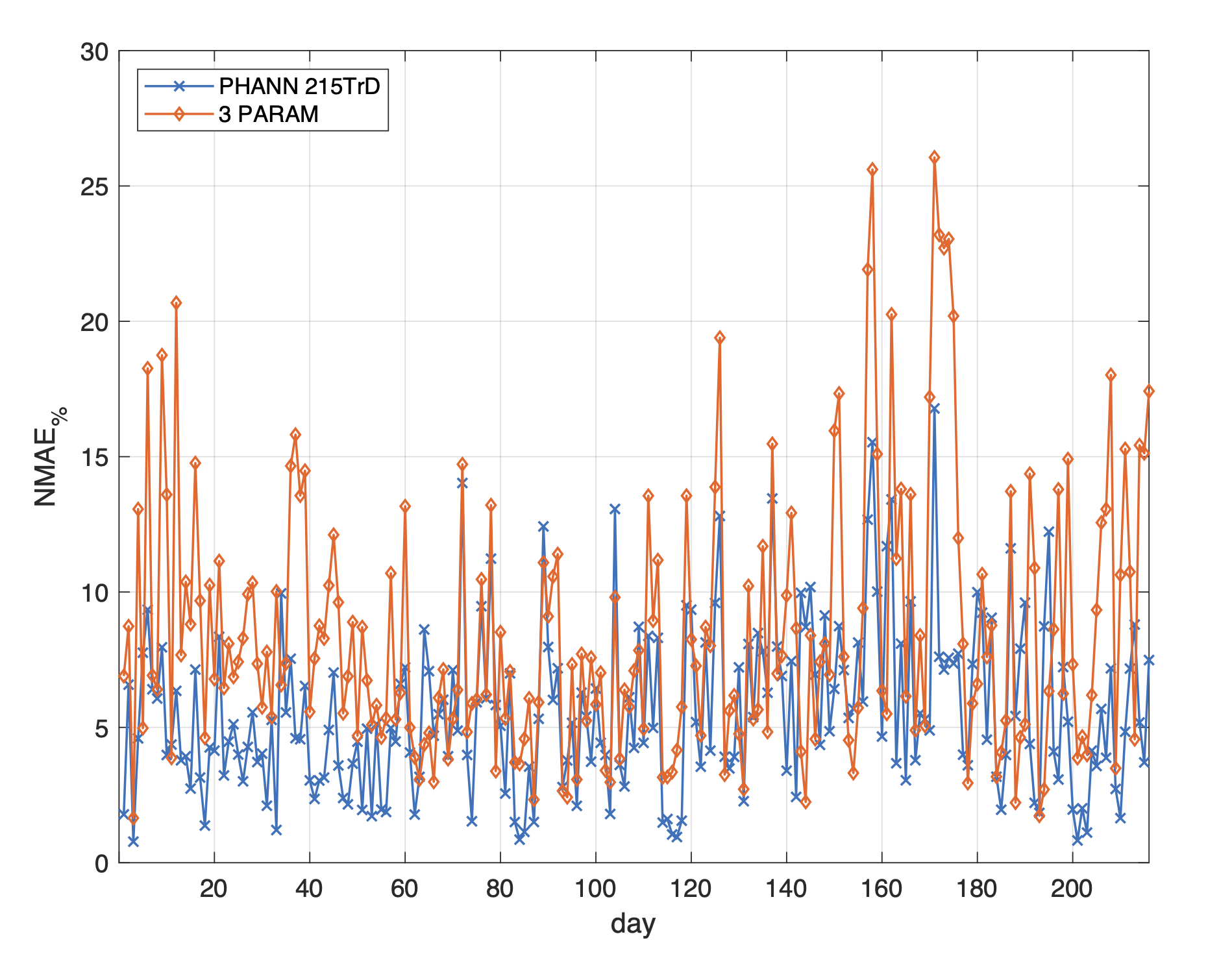
Figure 12: Daily NMAE% of the PHANN method trained with 10 days (left) and with 215 days (right) compared with the three-parameters model.

Dolara et al. (2018) analysed the effect of different approaches in the composition of a training data-set for the day-ahead forecasting of PV power production based on NN. In particular, the influence of different data-set compositions on the forecast outcome has been investigated by increasing the size of the training set size and by varying the lengths of the training and validation sets, in order to assess the most effective training method of this machine learning approach. As a general comment on the reported results, it can be stated that a method that employs the same chronologically consecutive samples for training is best suited when the availability of historical data is limited (for example, in newly deployed PV plant), while training based on randomly mixed samples method, appears to be most effective in the case of a greater data availability. Generally speaking, ensembles composed of independent trials are most effective.

3.4.9 Long-term simulation for large electrical power systems¹³¹

In large electrical power systems with renewable energy dependence, the power generators need to be scheduled to supply the system demand (Queiroz, 2016). In general, for modelling long-term renewables future behaviour, such as hydro, wind and solar photovoltaics (PV), stochastic scenarios should be included in the scheduling, usually in a dispatch optimisation problem under uncertainty – like described, for small systems, in §3.4.1 and, for wave forecasting, in §3.4.7. Due to the complexity and uncertainly associated, this problem is, in general, modelled with time series scenarios and multi-stage stochastic approaches. Queiroz (2016) presented a review for hydrothermal systems, with a focus on the optimisation algorithms. §3.4.6 and §3.4.8 explore the up-to-date methods for wind and PV solar power forecasting.

Here, we emphasise the importance of forecasting with simulation in the long-term renewable energy planning, especially in hydroelectric systems. In this context, due to the data spatial and temporal dependence structure, time series models are useful for future scenarios generation. Although the proposal could be forecasting for short-term planning and scheduling (as described in §3.4.6, 3.4.7, and §3.4.8), simulation strategies are explored for considering and estimating uncertainty in medium and/or long-term horizons.

According to Hipel & McLeod (1994), stochastic processes of natural phenomena, such as the renewables ones, are, in general, stationary. One of the main features of hydroelectric generation systems is the strong dependence on hydrological regimes. To deal with this task, the literature focuses on two main classes for forecasting/simulation streamflow data: physical and data-driven models (Zhang, Peng, Zhang, & Wang, 2015). Water resources management for hydropower generation and energy planning is one of the main challenges for decision-makers. At large, the hydrological data are transformed into the so-called affluent natural energy, that is used for scenarios simulation and serve as input for the optimisation algorithms (Oliveira, Souza, & Marcato, 2015). The current state-of-the-art models for this proposal are the periodic ones. Hipel & McLeod (1994) presented a wide range of possibilities, but the univariate periodic autoregressive (PAR, a periodic extension version of the ones presented in §2.3.4) is still the benchmark, with several enhanced versions. The approach fits a model to each period of the historical data and the residuals are simulated to generate new future versions of the time series, considered stationary. Among many others, important variations and alternative proposals to PAR with bootstrap procedures (see bootstrap details in §2.7.5), Bayesian dynamic linear models, spatial information and copulas versions (for copulas references, see §2.4.3) are detailed in Souza, Marcato, Dias, & Oliveira (2012), Marangon Lima, Popova, & Damien (2014), Lohmann, Hering, & Rebennack (2016) and Almeida Pereira & Veiga (2019), respectively.

It is worth considering the need for renewables portfolio simulation. This led Pinheiro Neto et al. (2017) to propose a model to integrate hydro, wind and solar power scenarios for Brazilian data. For the Eastern United States, Shahriari & Blumsack (2018) add to the literature on the wind, solar and blended portfolios over several spatial and temporal scales. For China, Liu et al. (2020) proposed a multi-variable model, with a unified framework, to simulate wind and PV scenarios to compensate hydropower generation. However, in light of the aforementioned, one of the key challenges and trends for renewable electrical power systems portfolio simulation are still related to the inclusion of exogenous variables, such as climate, meteorological, calendar and economic ones, as mentioned in §3.4.2.

3.4.10 Collaborative forecasting in the energy sector¹³²

As mentioned in §3.4.6, the combination of geographically distributed time series data, in a collaborative forecasting (or data sharing) framework, can deliver significant improvements in the forecasting accuracy of each individual renewable energy power plant. The same is valid for hierarchical load forecasting (Hong et al., 2019) and energy price forecasting (see §3.4.2). A review of multivariate time series forecasting methods can be found in §2.3.9 2.3.11 and §2.4.3. However, this data might have different owners, which are unwilling to share their data due to the following reasons: (i) personal or business sensitive information, (ii) lack of understanding about which data can and cannot be shared, and (iii) lack of information about economic (and technical) benefits from data sharing.

In order to tackle these limitations, recent research in energy time series forecasting is exploring two alternative (and potentially complementary) pathways: (i) privacy-preserving analytics, and (ii) data markets.

The role of privacy-preserving techniques applied collaborative forecasting is to combine time series data from multiple data owners in order to improve forecasting accuracy and keep data private at the same time. For solar energy forecasting, Berdugo, Chaussin, Dubus, Hebrail, & Leboucher (2011) described a method based on local and global analog-search that uses solar power time series from neighbouring sites, where only the timestamps and normalised weights (based on similarity) are exchanged and not the time series data. Y. Zhang & Wang (2018) proposed, for wind energy forecasting with spatia-temporal data, a combination of ridge linear quantile regression and Alternating Direction Method of Multipliers (ADMM) that enables each data owner to autonomously solve its forecasting problem, while collaborating with the others to improve forecasting accuracy. However, as demonstrated by C. Gonçalves et al. (2021a), the mathematical properties of these algorithms should be carefully analysed in order to avoid privacy breaches (i.e., when a third party recovers the original data without consent).

An alternative approach is to design a market (or auction) mechanism for time series or forecasting data where the data owners are willing to sell their private (or confidential) data in exchange for an economic compensation (Agarwal, Dahleh, & Sarkar, 2019). The basic concept consists in pricing data as a function of privacy loss, but it can be also pricing data as a function of tangible benefits such as electricity market profit maximization. C. Gonçalves et al. (2021b) adapted for renewable energy forecasting the model described in Agarwal et al. (2019), by considering the temporal nature of the data and relating data price with the extra revenue obtained in the electricity market due to forecasting accuracy improvement. The results showed a benefit in terms of higher revenue resulting from the combination of electricity and data markets. With the advent of peer-to-peer energy markets at the domestic consumer level (Parag & Sovacool, 2016), smart meter data exchange between peers is also expected to increase and enable collaborative forecasting schemes. For this scenario, Yassine, Shirehjini, & Shirmohammadi (2015) proposed a game theory mechanism where a energy consumer maximizes its reward by sharing consumption data and a data aggregator can this data with a data analyst (which seeks data with the lowest possible price).

Finally, promoting data sharing via privacy-preserving or data monetisation can also solve data scarcity problems in some use cases of the energy sector, such as forecasting the condition of electrical grid assets (Fan, Nowaczyk, & Röognvaldsson, 2020). Moreover, combination of heterogeneous data sources (e.g., numerical, textual, categorical) is a challenging and promising avenue of future research in collaborative forecasting (Obst et al., 2019).

3.5 Environmental applications

3.5.1 Forecasting two aspects of climate change¹³³

First into the Industrial Revolution, the UK is one of the first out: in 2013 its per capita CO\(_2\) emissions dropped below their 1860 level, despite per capita real incomes being around 7-fold higher (Hendry, 2020). The model for forecasting UK CO\(_2\) emissions was selected from annual data 1860-2011 on CO\(_2\) emissions, coal and oil usage, capital and GDP, their lags and non-linearities (see §3.5.2 for higher frequency weather forecasts). Figures 13(a) to 13(c) show the non-stationary time series with strong upward then downward trends, punctuated by large outliers from world wars, miners strikes plus shifts from legislation and technological change: J. L. Castle & Hendry (2020). Saturation estimation at 0.1% using Autometrics (Doornik, 2018) retaining all other regressors, detected 4 step shifts coinciding with major policy interventions like the 2008 Climate Change Act, plus numerous outliers, revealing a cointegrated relation. The multi-step forecasts over 2012—2017 from a VAR in panel (d) of Figure 13 show the advantage of using step-indicator saturation (SIS: Castle et al., 2015b).

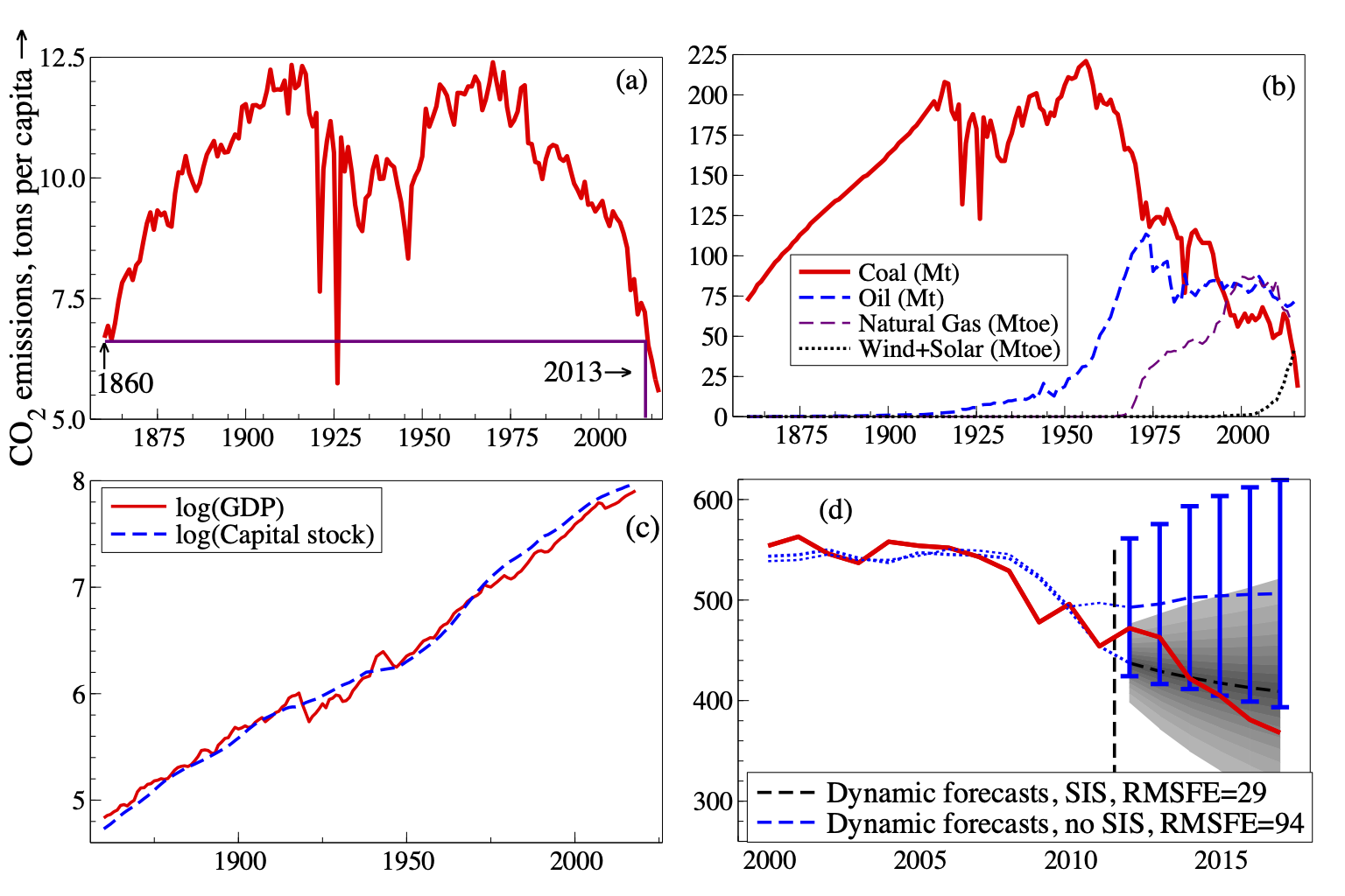
Figure 13: (a) UK emissions, (b) energy sources in megatonnes (Mt) and megatonnes of oil equivalent (Mtoe), (c) economic variables, and (d) multi-step forecasts of CO2 emissions in Mt.

We formulated a 3-equation simultaneous model of atmospheric CO\(_2\) and Antarctic Temperature and Ice volume over 800,000 years of Ice Ages in 1000-year frequency (Kaufmann & Juselius, 2013; Paillard, 2001). Driven by non-linear functions of eccentricity, obliquity, and precession (see panels (a), (b), and (c) of Figure 14 respectively), the model was selected with saturation estimation. Earth’s orbital path is calculable into the future ((Croll, 1875) and (Milankovitch, 1969)), allowing 100,000 years of multi-step forecasts at endogenous emissions. Humanity has affected climate since 10 thousand years ago (kya: Ruddiman (2005)), so we commence forecasts there. Forecasts over \(-10\) to 100 with time series from 400kya in panels (d) to (f) of Figure 14 show paths within the ranges of past data $$2.2SE (Pretis & Kaufmann, 2018).

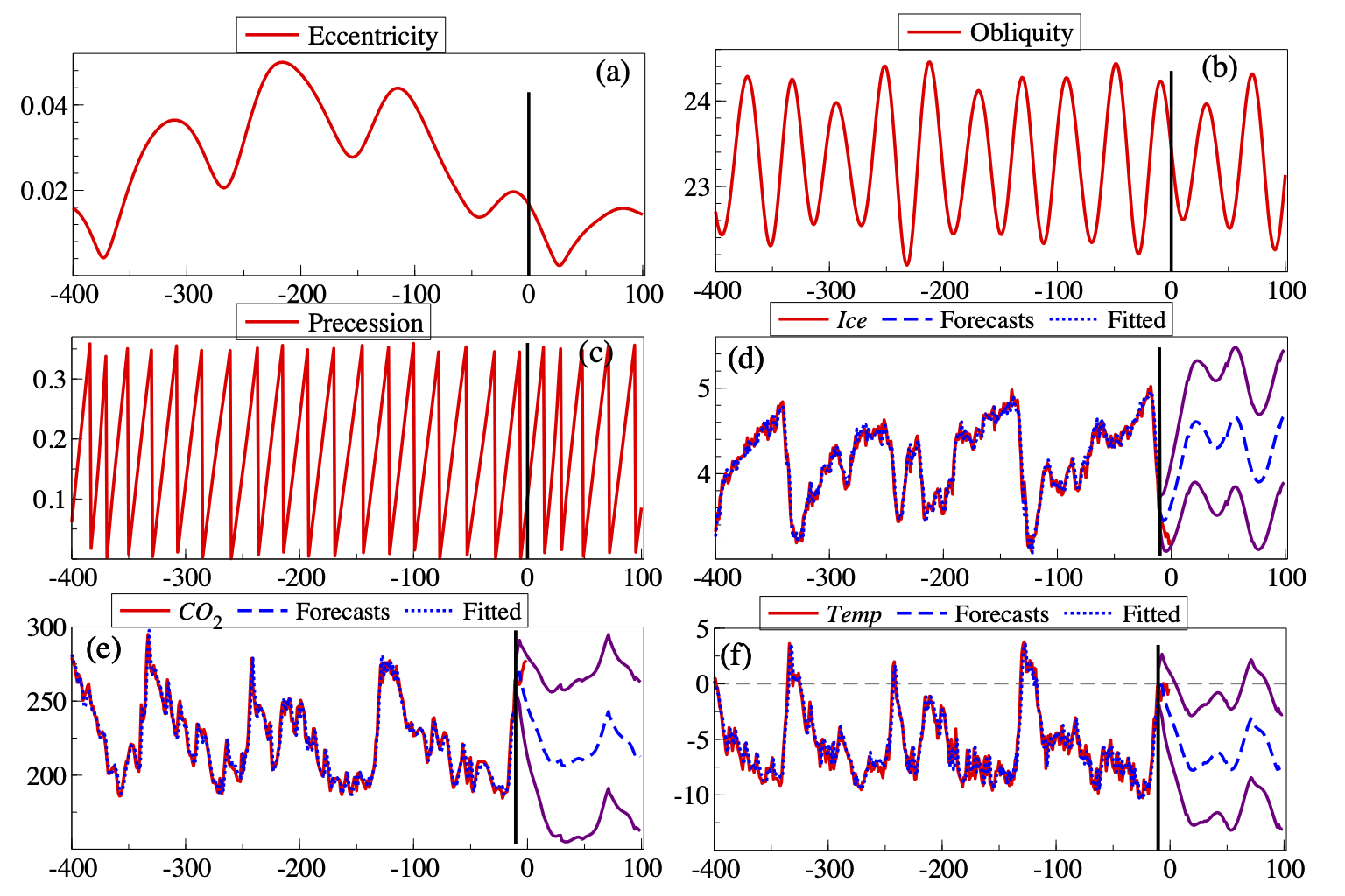
Figure 14: Ice-Age data, model fits, and forecasts with endogenous CO₂.

Atmospheric CO\(_2\) already exceeds 400ppm (parts per million), dramatically outside the Ice-Age range (Sundquist & Keeling, 2009). Consequently, we conditionally forecast the next 100,000 years, simulating the potential climate for anthropogenic CO\(_2\) (J. L Castle & Hendry, 2020) noting the ‘greenhouse’ temperature is proportional to the logarithm of CO\(_2\) ((Arrhenius, 1896)). The orbital drivers will continue to influence all three variables but that relation is switched off in the scenario for ‘exogenised’ CO\(_2\). The 110 dynamic forecasts conditional on 400ppm and 560ppm with ±2SE bands are shown in Figure 15, panels (a) and (b) for Ice and Temperature respectively. The resulting global temperature rises inferred from these Antarctic temperatures would be dangerous, at more than 5\(^{\circ}\)C, with Antarctic temperatures positive for thousands of years (Pretis & Kaufmann, 2020; Vaks, Mason, Breitenbach, & al., 2019).

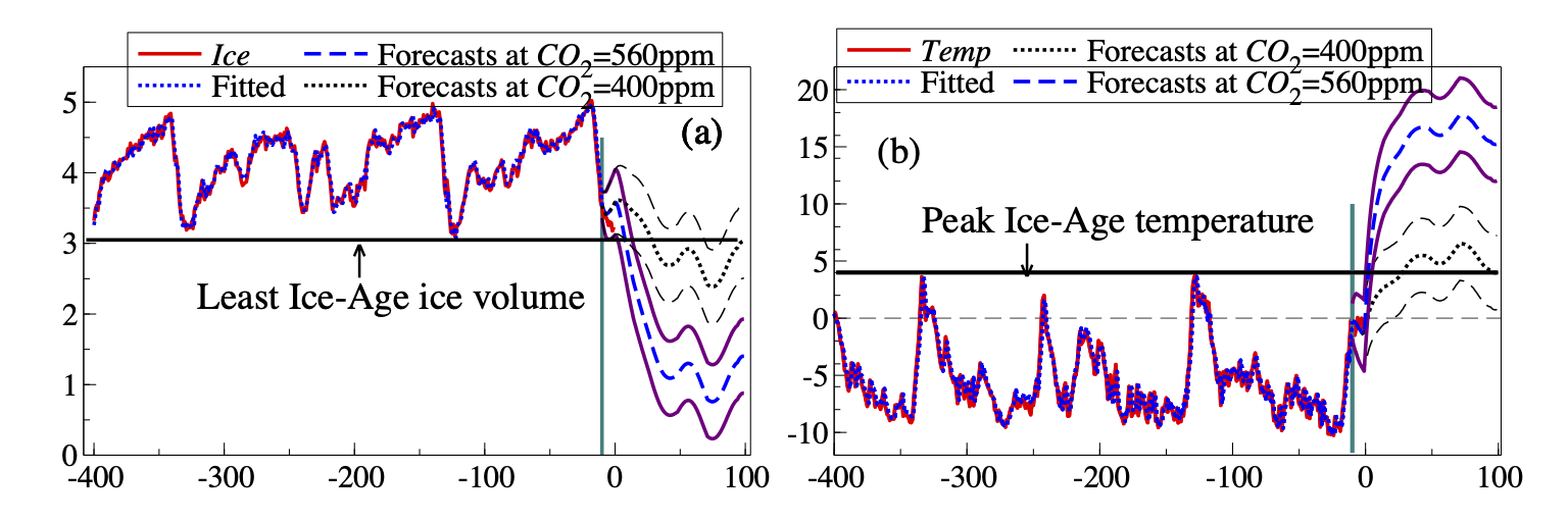
Figure 15: Ice-Age simulations with exogenous CO₂.

3.5.2 Weather forecasting¹³⁴

The weather has a huge impact on our lives, affecting health, transport, agriculture (see also §3.8.10), energy use (see also §3.4), and leisure. Since Bjerknes (1904) introduced hydrodynamics and thermodynamics into meteorology, weather prediction has been based on merging physical principles and observational information. Modern weather forecasting is based on numerical weather prediction (NWP) models that rely on accurate estimates of the current state of the climate system, including ocean, atmosphere and land surface. Uncertainty in these estimates is propagated through the NWP model by running the model for an ensemble of perturbed initial states, creating a weather forecast ensemble (Buizza, 2018; Toth & Buizza, 2019).

One principal concern in NWP modelling is that small-scale phenomena such as clouds and convective precipitation are on too small a scale to be represented directly in the models and must, instead, be represented by approximations known as parameterisations. Current NWP model development aims at improving both the grid resolution and the observational information that enters the models (Bannister, Chipilski, & Martinez-Alvarado, 2020; Leuenberger et al., 2020). However, for fixed computational resources, there is a trade-off between grid resolution and ensemble size, with a larger ensemble generally providing a better estimate of the prediction uncertainty. Recent advances furthermore include machine learning approaches (see §2.7.10) to directly model the small-scale processes, in particular cloud processes (see, for example, Gentine, Pritchard, Rasp, Reinaudi, & Yacalis, 2018; Rasp, Pritchard, & Gentine, 2018).

Despite rapid progress in NWP modelling, the raw ensemble forecasts exhibit systematic errors in both magnitude and spread (Buizza, 2018). Statistical post-processing is thus routinely used to correct systematic errors in calibration and accuracy before a weather forecast is issued; see Vannitsem, Wilks, & Messner (2018) for a recent review but also §2.12.4 and §2.12.5. A fundamental challenge here is to preserve physical consistency across space, time and variables (see, for example, Möller, Lenkoski, & Thorarinsdottir, 2013; Claudio Heinrich et al., 2020; Schefzik, Thorarinsdottir, & Gneiting, 2013). This is particularly important when the weather forecast is used as input for further prediction modelling, e.g., in hydrometeorology (Hemri, 2018; Hemri, Lisniak, & Klein, 2015).

At time scales beyond two weeks, the weather noise that arises from the growth of the initial uncertainty, becomes large (Royer, 1993). Sources of long-range predictability are usually associated with the existence of slowly evolving components of the earth system, including the El Niño Southern Oscillation (ENSO), monsoon rains, the Madden Julian Oscillation (MJO), the Indian Ocean dipole, and the North Atlantic Oscillation (NAO), spanning a wide range of time scales from months to decades (Hoskins, 2013; Vitart, Robertson, & Anderson, 2012). It is expected that, if a forecasting system is capable of reproducing these slowly evolving components, they may also be able to forecast them (Van Schaeybroeck & Vannitsem, 2018). The next step is then to find relationships between modes of low-frequency variability and the information needed by forecast users such as predictions of surface temperature and precipitation (Roulin & Vannitsem, 2019; Smith et al., 2020).

3.5.3 Air quality forecasting¹³⁵

To preserve human health, European Commission stated in the Directive (2008/50/EC) that member states have to promptly inform the population when the particulate matter (PM) daily mean value exceeds (or is expected to exceed) the threshold of \(50 \mu g/m^3\). Therefore, systems have been designed in order to produce forecasts for up to three days in advance using as input the measured value of concentration and meteorological conditions. These systems can be classified in (i) data-driven models (Carnevale, Finzi, Pisoni, & Volta, 2016; Corani, 2005 and §2.7; Stadlober, Hormann, & Pfeiler, 2018), and (ii) deterministic chemical and transport models (Honoré et al., 2007; Manders, Schaap, & Hoogerbrugge, 2009). In this section, a brief overview of the application of these systems to the high polluted area of Lombardy region, in Italy, will be presented.

Carnevale, Finzi, Pederzoli, Turrini, & Volta (2018) compared the results of three different forecasting systems based on neural networks, lazy learning models, and regression trees respectively. A single model has been identified for each monitoring station. In the initial configuration, only the last three PM measurements available were used to produce the forecast. In this configuration, the systems offered reasonable performance, with correlation coefficients ranging from 0.6 (lazy learning method) to 0.75 (neural network). The work also demonstrated that the performance of the ensemble of the three systems was better than the best model for each monitoring station (see also §2.6 for further discussions on forecast combinations).

Starting from the results of this work, a second configuration was implemented, using as input also the wind speed measured in the meteorological monitoring station closest to the measurement point of PM. The researchers observed an improvement in all performance indices, with the median of the correlation for the best model (neural networks) increasing from 0.75 to 0.82 and the RMSE dropping from \(15 \mu g/m^3\) to \(7 \mu g/m^3\).

One of the main drawbacks of data-driven models for air quality is that they provide information only in the point where the measurements are available. To overcome this limitation, recent literature has presented mixed deterministic and data-driven approaches (see, for example, Carnevale, Angelis, Finzi, Turrini, & Volta, 2020) which use the data assimilation procedure and offer promising forecasting performance.

From a practical point of view, critical issues regarding forecasting air quality include:

• Information collection and data access: even if regional authorities have to publicly provide data and information related to air quality and meteorology, the measured data are not usually available in real-time and the interfaces are sometimes not automated;

• Data quantity: the amount of information required by air quality forecasting systems is usually large, in particular towards the definition of the training and validation sets;

• Non-linear relationships: the phenomenon of accumulation of pollutants in atmosphere is usually affected by strong nonlinearities, which significantly impact the selection of the models and their performance;

• Unknown factors: it is a matter of fact that the dynamic of pollutants in atmosphere is affected by a large number of non-measurable variables (such as meteorological variables or the interaction with other non-measurable pollutants), largely affecting the capability of the models to reproduce the state of the atmosphere.

3.5.4 Forecasting and decision making for floods and water resources management¹³⁶

In Water Resources and Flood Risk Management, decision makers are frequently confronted with the need of taking the most appropriate decisions not knowing what will occur in the future. To support their decision-making under uncertainty, decision theory (Berger, 1985; Bernardo, 1994; DeGroot, 2004) invokes Bayesian informed decision approaches, which find the most appropriate decision by maximising (or minimising) the expected value of a “utility function”, thus requiring its definition, together with the estimation of a “predictive probability” density (Berger, 1985) due to the fact that utility functions are rarely linear or continuous. Consequently, their expected value does not coincide with the value assumed on the predicted “deterministic” expected value. Accordingly, overcoming the classical 18^th century “mechanistic” view by resorting into probabilistic forecasting approaches becomes essential (see also §2.6.2).

The failure of decision-making based on deterministic forecasts in the case of Flood Risk Management is easily shown through a simple example. At a river section, the future water level provided by a forecast is uncertain and can be described by a Normal distribution with mean 10 meters and standard deviation of 5 meters. Given a dike elevation of 10.5 meters, damages may be expected as zero if water level falls below the dike elevation and linearly growing when level exceeds it with a factor of \(10^6\) dollars. If one assumes the expect value of forecast as the deterministic prediction to compute the damage the latter will result equal to zero, while if one correctly integrates the damage function times the predictive density the estimated expected damage will results into 6.59 millions of dollars and educated decisions on alerting or not the population or evacuating or not a flood-prone area can be appropriately taken (see also §3.6).

Water resources management, and in particular reservoirs management, aim at deriving appropriate operating rules via long term expected benefits maximisation. Nonetheless, during flood events decision makers must decide how much to preventively release from multi-purpose reservoirs in order to reduce dam failure and downstream flooding risks the optimal choice descending from trading-off between loosing future water resource vs the reduction of short term expected losses.

This is obtained by setting up an objective function based on the linear combination of long and short term “expected losses”, once again based on the available probabilistic forecast. This Bayesian adaptive reservoir management approach incorporating into the decision mechanism the forecasting information described by the short-term predictive probability density, was implemented on the lake Como since 1997 (Todini, 1999, 2017) as an extension of an earlier original idea (Todini, 1991). This resulted into:

• a reduction of over 30% of of the city of Como frequency;

• an average reduction of 12% of the water deficit;

• an increase of 3% in the electricity production.

Lake Como example clearly shows that instead of basing decisions on the deterministic prediction, the use of a Bayesian decision scheme, in which model forecasts describe the predictive probability density, increases the reliability of the management scheme by essentially reducing the probability of wrong decisions (Todini, 2017, 2018).

3.6 Social good and demographic forecasting

3.6.1 Healthcare¹³⁷

There are many decisions that depend on the quality of forecasts in the health care system, from capacity planning to layout decisions to the daily schedules. In general, the role of forecasting in health care is to inform both clinical and non-clinical decisions. While the former concerns decisions related to patients and their treatments (Makridakis et al., 2019), the latter involves policy/management, and supply chain decisions that support the delivery of high-quality care for patients.

A number of studies refer to the use of forecasting methods to inform clinical decision making. These methods are used to screen high risk patients for preventative health care (Chen, Wang, & Hung, 2015; Mark et al., 2014; Santos, Abreu, Garca-Laencina, Simão, & Carvalho, 2015; Uematsu, Kunisawa, Sasaki, Ikai, & Imanaka, 2014), to predict mental health issues (Shen et al., 2017; Tran et al., 2013), to assist diagnosis and disease progression (Ghassemi et al., 2015; F. Ma et al., 2017; Pierce et al., 2010; Qiao, Wu, Ge, & Fan, 2019), to determine prognosis (Dietzel et al., 2010; Ng, Stein, Ning, & Black-Schaffer, 2007), and to recommend treatments for patients (Kedia & Williams, 2003; Scerri et al., 2006; Shang, Ma, Xiao, & Sun, 2019). Common forecasting methods to inform clinical decisions include time series (see §2.3.1, §2.3.4, and §2.3.5), regression (see §2.3.2), classification tree (see §2.7.12), neural networks (see §2.7.8), Markov models (see §2.3.12) and Bayesian networks. These models utilise structured and unstructured data including clinician notes (Austin & Kusumoto, 2016; Labarere, Bertrand, & Fine, 2014) which makes the data pre-processing a crucial part of the forecasting process in clinical health care.

One of the aspects of the non-clinical forecasting that has received the most attention in both research and application is the policy and management. Demand forecasting is regularly used in Emergency Departments (Arora, Taylor, & Mak, 2020; Choudhury & Urena, 2020; Khaldi, El Afia, & Chiheb, 2019; Rostami-Tabar & Ziel, 2020), ambulance services (Al-Azzani, Davari, & England, 2020; Setzler, Saydam, & Park, 2009; Vile, Gillard, Harper, & Knight, 2012; Zhou & Matteson, 2016) and hospitals with several different specialities (McCoy, Pellegrini, & Perlis, 2018; Ordu, Demir, & Tofallis, 2019; Zhou, Zhao, Wu, Cheng, & Huang, 2018) to inform operational, tactical and strategic planning. The common methods used for this purpose include classical ARIMA and exponential smoothing methods, regression, singular spectrum analysis, Prophet, Double-Seasonal Holt-Winter, TBATS and Neural Networks. In public health, forecasting can guide policy and planning. Although it has a wider definition, the most attention is given to Epidemic forecasting (see also §3.6.2).

Forecasting is also used in both national and global health care supply chains, not only to ensure the availability of medical products for the population but also to avoid excessive inventory. Additionally, the lack of accurate demand forecast in a health supply chain may cost lives (Baicker, Chandra, & Skinner, 2012) and has exacerbated risks for suppliers (Levine, Pickett, Sekhri, & Yadav, 2008). Classical exponential smoothing, ARIMA, regression and Neural Network models have been applied to estimate the drug utilisation and expenditures (Dolgin, 2010; Linnér, Eriksson, Persson, & Wettermark, 2020), blood demand (Fortsch & Khapalova, 2016), hospital supplies (Gebicki, Mooney, Chen, & Mazur, 2014; Riahi, Hosseini-Motlagh, & Teimourpour, 2013) and demand for global medical items (Amarasinghe, Wichmann, Margolis, & Mahoney, 2010; Hecht & Gandhi, 2008; Laan, Dalen, Rohrmoser, & Simpson, 2016). It is important to note that, while the demand in a health care supply chain has often grouped and hierarchical structures (Mircetica, Rostami-Tabar, Nikolicica, & Maslarica, 2020 see also §2.10.1), this has not been well investigated and needs more attention.

3.6.2 Epidemics and pandemics¹³⁸

Pandemics and epidemics both refer to disease outbreaks. An epidemic is a disease outbreak that spreads across a particular region. A pandemic is defined as spread of a disease worldwide. Forecasting the evolution of a pandemic or an epidemic, the growth of cases and fatalities for various horizons and levels of granularity, is a complex task with raw and limited data – as each disease outbreak type has unique features with several factors affecting the severity and the contagiousness. Be that as it may, forecasting becomes an paramount task for the countries to prepare and plan their response (Nikolopoulos, 2020), both in healthcare and the supply chains (Beliën & Forcé, 2012 see also §3.6.1 and §3.2.2).

Successful forecasting methods for the task include time-series methods (see §2.3), epidemiological and agent-based models (see §2.7.3), metapopulation models, approaches in metrology (Nsoesie, Mararthe, & Brownstein, 2013), machine and deep learning methods (Yang et al., 2020). Andersson et al. (2008) used regression models for the prediction of the peak time and volume of cases for a pandemic with evidence from seven outbreaks in Sweden. Yaffee et al. (2011) forecasted the evolution of the Hantavirus epidemic in USA and compared causal and machine-learning methods with time-series methods and found that univariate methods quite successful. Soebiyanto, Adimi, & Kiang (2010) used ARIMA models for successfully short-term forecasting of influenza weekly cases. Shaman & Karspeck (2012) used Kalman filter based SIR epidemiological models to forecast the peak time of influenza 6-7 weeks ahead.

For COVID-19, Petropoulos & Makridakis (2020) applied a multiplicative exponential smoothing model (see also §2.3.1) for predicting global number of confirmed cases, with very successful results both for point forecasts and prediction intervals. This article got serious traction with 100,000 views and 300 citations in the first twelve months since its publication, thus evidencing the importance of such empirical investigations. There has been a series of studies focusing on predicting deaths in the USA and European countries for the first wave of the COVID-19 pandemic (IHME COVID-19 health service utilization forecasting team & Murray, 2020a, 2020b). Furthermore, Petropoulos et al. (2020) expanded their investigation to capture the continuation of both cases and deaths as well as their uncertainty, achieving high levels of forecasting accuracy for ten-days-ahead forecasts over a period of four months. Along the same lines, Doornik et al. (2020b) have been publishing real-time accurate forecasts of confirmed cases and deaths from mid-March 2020 onwards. Their approach is based on extraction of trends from the data using machine learning.

Pinson & Makridakis (2020) organised a debate between Taleb and Ioannidis on forecasting pandemics. Ioannidis, Cripps, & Tanner (2020) claim that forecasting for COVID-19 has by and large failed. However they give recommendations of how this can be averted. They suggest that the focus should be on predictive distributions and models should be continuously evaluated. Moreover, they emphasise the importance of multiple dimensions of the problem (and its impact). Taleb et al. (2020) discuss the dangers of using naive, empirical approaches for fat-tailed variables and tail risk management. They also reiterate the inefficiency of point forecasts for such phenomena.

Finally, Nikolopoulos et al. (2020) focused on forecast-driven planning, predicting the growth of COVID-19 cases and the respective disruptions across the supply chain at country level with data from the USA, India, UK, Germany, and Singapore. Their findings confirmed the excess demand for groceries and electronics, and reduced demand for automotive – but the model also proved that the earlier a lock-down is imposed, the higher the excess demand will be for groceries. Therefore, governments would need to secure high volumes of key products before imposing lock-downs; and, when this is not possible, seriously consider more radical interventions such as rationing.

Dengue is one of the most common epidemic diseases in tropical and sub-tropical regions of the world. Estimates of World Health Organisation reveals that about half of the world’s population is now at risk for Dengue infection (Romero, Olivero, Real, & Guerrero, 2019). Aedes aegypti and Aedes albopictus are the principal vectors of dengue transmission and they are highly domesticated mosquitoes. Rainfall, temperature and relative humidity are thought of as important factors attributing towards the growth and dispersion of mosquito vectors and potential of dengue outbreaks (Banu, Hu, Hurst, & Tong, 2011).

In reviewing the existing literature, two data types have been used to forecast dengue incidence: (i) spatio-temporal data: incidence of laboratory-confirmed dengue cases among the clinically suspected patients (Naish et al., 2014), (ii) web-based data: Google trends, tweets associated with Dengue cases (Almeida Marques-Toledo et al., 2017).

SARIMA models (see also §2.3.4) have been quite popular in forecasting laboratory-confirmed dengue cases (Gharbi et al., 2011; Martinez & Silva, 2011; Promprou, Jaroensutasinee, & Jaroensutasinee, 2006). Chakraborty, Chattopadhyay, & Ghosh (2019) used a hybrid model combining ARIMA and neural network autoregressive (NNAR) to forecast dengue cases. In light of biological relationships between climate and transmission of Aedes mosquitoes, several studies have used additional covariates such as, rainfall, temperature, wind speed, and humidity to forecasts dengue incidence (Banu et al., 2011; Naish et al., 2014; Talagala, 2015). Poisson regression model has been widely used to forecast dengue incidence using climatic factors and lagged time between dengue incidence and weather variables (Hii, Zhu, Ng, Ng, & Rocklöv, 2012; Koh, Spindler, Sandgren, & Jiang, 2018). Several researchers looked at the use of Quasi‐Poisson and negative binomial regression models to accommodate over dispersion in the counts (Lowe et al., 2011; C. Wang et al., 2014). Cazelles, Chavez, McMichael, & Hales (2005) used wavelet analysis to explore the dynamic of dengue incidence and wavelet coherence analyses was used to identify time and frequency specific association with climatic variables. Almeida Marques-Toledo et al. (2017) took a different perspective and look at weekly tweets to forecast Dengue cases. Rangarajan, Mody, & Marathe (2019) used Google trend data to forecast Dengue cases. Authors hypothesised that web query search related to dengue disease correlated with the current level of dengue cases and thus may be helpful in forecasting dengue cases.

A direction for future research in this field is to explore the use of spatio-temporal hierarchical forecasting (see §2.10).

3.6.3 Forecasting mortality¹³⁹

Actuarial, Demographic, and Health studies are some examples where mortality data are commonly used. A valuable source of mortality information is the Human Mortality Database (HMD), a database that provides mortality and population data for 41 mainly developed countries. Additionally, at least five country-specific databases are devoted to subnational data series: Australian, Canadian, and French Human Mortality Databases, United States and Japan Mortality Databases. In some situations, the lack of reliable mortality data can be a problem, especially in developing countries, due to delays in registering or miscounting deaths (Checchi & Roberts, 2005). Analysis of National Causes of Death for Action (ANACONDA) is a valuable tool that assesses the accuracy and completeness of data for mortality and cause of death by checking for potential errors and inconsistencies (Mikkelsen, Moesgaard, Hegnauer, & Lopez, 2020).

The analysis of mortality data is fundamental to public health authorities and policymakers to make decisions or evaluate the effectiveness of prevention and response strategies. When facing a new pandemic, mortality surveillance is essential for monitoring the overall impact on public health in terms of disease severity and mortality (Setel et al., 2020; Vestergaard et al., 2020). A useful metric is excess mortality and is the difference between the observed number of deaths and the expected number of deaths under “normal” conditions (Aron & Muellbauer, 2020; Checchi & Roberts, 2005). Thus, it can only be estimated with accurate and high-quality data from previous years. Excess mortality has been used to measure the impact of heat events (Limaye, Vargo, Harkey, Holloway, & Patz, 2018; Matte, Lane, & Ito, 2016), pandemic influenza (Nielsen et al., 2013; Nunes et al., 2011), and nowadays COVID-19 (Nogueira, Araújo Nobre, Nicola, Furtado, & Carneiro, 2020; Ritchie et al., 2020; Shang & Xu, 2021 and §3.6.2; Sinnathamby et al., 2020), among others. Excess mortality data have been making available by the media publications The Economist, The New York Times and The Financial Times. Moreover, a monitoring system of the weekly excess mortality in Europe has been performed by the EuroMOMO project (Vestergaard et al., 2020).

An essential use of mortality data for those individuals at age over 60 is in the pension and insurance industries, whose profitability and solvency crucially rely on accurate mortality forecasts to adequately hedge longevity risks (see, e.g., Shang & Haberman, 2020a, 2020b). Longevity risk is a potential systematic risk attached to the increasing life expectancy of annuitants, and it is an important factor to be considered when determining a sustainable government pension age (see, e.g., R. J. Hyndman et al., 2021 for Australia). The price of a fixed-term or lifelong annuity is a random variable, as it depends on the value of zero-coupon bond price and mortality forecasts. The zero-coupon bond price is a function of interest rate (see §3.3.6) and is comparably more stable than the retirees’ mortality forecasts.

Several methodologies were developed for mortality modelling and forecasting (Booth & Tickle, 2008; Janssen, 2018). These methods can be grouped into three categories: expectation, explanation, and extrapolation (Booth & Tickle, 2008).

The expectation approach is based on the subjective opinion of experts (see also §2.11.4), who set a long-run mortality target. Methods based on expectation make use of experts’ opinions concerning future mortality or life expectancy with a specified path and speed of progression towards the assumed value (Continuous Mortality Investigation, 2020). The advantage of this approach is that demographic, epidemiological, medical, and other relevant information may be incorporated into the forecasts. The disadvantages are that such information is subjective and biased towards experts’ opinions, and it only produces scenario-based (see §2.11.5) deterministic forecasts (Ahlburg & Vaupel, 1990; Wong-Fupuy & Haberman, 2004).

The explanation approach captures the correlation between mortality and the underlying cause of death. Methods based on the explanation approach incorporate medical, social, environmental, and behavioural factors into mortality modelling. Example include smoking and disease-related mortality models. The benefit of this approach is that mortality change can be understood from changes in related explanatory variables; thus, it is attractive in terms of interpretability (Gutterman & Vanderhoof, 1998).

The extrapolative approach is considered more objective, easy to use and more likely to obtain better forecast accuracy than the other two approaches (Janssen, 2018). The extrapolation approach identifies age patterns and trends in time which can be then forecasted via univariate and multivariate time series models (see §2.3). In the extrapolation approach, many parametric and nonparametric methods have been proposed (see, e.g., Alho & Spencer, 2005; Hyndman & Ullah, 2007; Shang, Booth, & Hyndman, 2011). Among the parametric methods, the method of Heligman & Pollard (1980) is well-known. Among the nonparametric methods, the Lee-Carter model (Lee & Carter, 1992), Cairns-Blake-Dowd model (Cairns et al., 2009; Dowd et al., 2010), and functional data model (Hyndman & Ullah, 2007 and §2.3.10), as well as their extensions and generalisations are dominant. The time-series extrapolation approach has the advantage of obtaining a forecast probability distribution rather than a deterministic point forecast and, also, enable the determination of forecast intervals (Booth & Tickle, 2008).

Janssen (2018) presents a review of the advances in mortality forecasting and possible future research challenges.

3.6.4 Forecasting fertility¹⁴⁰

Aside from being a driver of population forecasts (see §2.3.7), fertility forecasts are vital for planning maternity services and anticipating demand for school places. The key challenge relates to the existence of, and interaction between, the quantum (how many?) and tempo (when?) components (Booth, 2006). This intrinsic dependence on human decisions means that childbearing behaviour is influenced by numerous factors acting at different levels, from individual characteristics to societal change (Balbo, Billari, & Mills, 2013). An important methodological challenge for many low- and middle-income countries is fertility estimation, due to deficiencies in vital statistics caused by inadequate birth registration systems (AbouZahr et al., 2015; Moultrie et al., 2013; Phillips, Adair, & Lopez, 2018). Such countries are often also in the process of transitioning from high to low fertility, which induces greater forecast uncertainty compared to low-fertility countries (United Nations Development Programme, 2019).

A range of statistical models have been proposed to forecast fertility – see Booth (2006), Bohk-Ewald, Li, & Myrskylä (2018), and Shang & Booth (2020) for reviews. The Lee-Carter model (Lee & Carter, 1992) originally developed for mortality forecasting (see §3.6.3) has been applied to fertility (Lee, 1993), with extensions in functional data (Hyndman & Ullah, 2007) and Bayesian (Wiśniowski, Smith, Bijak, Raymer, & Forster, 2015) contexts. Other notable extrapolative methods include the cohort-ARIMA model of De Beer (1985, 1990) – see §2.3.4 – and the linear extrapolation method of Myrskylä, Goldstein, & Cheng (2013). Many parametric models have been specified to describe the shapes of fertility curves (Brass, 1974; Evans, 1986; Hoem et al., 1981; Schmertmann, 2003), with forecasts obtained through time series extrapolations of the parameters (Congdon, 1990; De Iaco & Maggio, 2016; Knudsen, McNown, & Rogers, 1993). Bayesian methods have been used to borrow strength across countries (for example, Alkema et al., 2011; Schmertmann, Zagheni, Goldstein, & Myrskylä, 2014), with Ellison, Dodd, & Forster (2020) developing a hierarchical model in the spirit of the latter. The top-down approach (see §2.10.1) of the former, which is used by the United Nations, projects the aggregate Total Fertility Rate (TFR) measure probabilistically (also see Tuljapurkar & Boe, 1999) before decomposing it by age. Hyppöla, Tunkelo, & Törnqvist (1949) provide one of the earliest known examples of probabilistic fertility forecasting (Alho & Spencer, 2005).

Little work has been done to compare forecast performance across this broad spectrum of approaches. The study of Bohk-Ewald et al. (2018) is the most comprehensive to date. Most striking is their finding that few methods can better the naive freezing of age-specific rates, and those that can differ greatly in method complexity (see also §2.5.2). A recent survey of fertility forecasting practice in European statistical offices (Gleditsch & Syse, 2020) found that forecasts tend to be deterministic and make use of expert panels (see §2.11.4). Expert elicitation techniques are gaining in sophistication, highlighted by the protocol of Statistics Canada (Dion, Galbraith, & Sirag, 2020) which requests a full probability distribution of the TFR.

A promising avenue is the development of forecasting methods that incorporate birth order (parity) information, supported by evidence from individual-level analyses (for example, Fiori, Graham, & Feng, 2014). Another underexplored area is the integration of survey data into fertility forecasting models, which tend to use vital statistics alone when they are of sufficient quality (see Rendall, Handcock, & Jonsson, 2009; Zhang & Bryant, 2019 for Bayesian fertility estimation with imperfect census data). Alternative data sources also have great potential. For example, Wilde, Chen, & Lohmann (2020) use Google data to predict the effect of COVID-19 on US fertility in the absence of vital statistics. Lastly, investigation of the possible long-term impacts of delayed motherhood in high-income countries, alongside developments in assisted reproduction technology such as egg freezing, is required (see, for example, Sobotka & Beaujouan, 2018).

3.6.5 Forecasting migration¹⁴¹

Migration forecasts are needed both as crucial input into population projections (see §2.3.7), as well as standalone predictions, made for a range of users, chiefly in the areas of policy and planning. At the same time, migration processes are highly uncertain and complex, with many underlying and interacting drivers, which evade precise conceptualisation, definitions, measurement, and theoretical description (Bijak & Czaika, 2020). Given the high level of the predictive uncertainty, and the non-stationary character of many migration processes (Bijak & Wiśniowski, 2010), the current state of the art of forward-looking migration studies reflects therefore a shift from prediction to the use of forecasts as contingency planning tools (idem).

Reviews of migration forecasting methods are available in Bijak (2010) and Sohst, Tjaden, Valk, & Melde (2020). The applications in official statistics, with a few exceptions, are typically based on various forms scenario-based forecasting with judgment (see §2.11.5), based on pre-set assumptions (for an example, see Abel, 2018). Such methods are particularly used for longer time horizons, of a decade or more, so typically in the context of applications in population projections, although even for such long time horizons calibrated probabilistic methods have been used as well (Azose et al., 2016).

The mainstream developments in migration forecasting methodology, however, include statistical and econometric methods discussed in §2.3, such as time series models, both uni- and multivariate (for example, Gorbey, James, & Poot, 1999; Bijak, 2010; Bijak et al., 2019), econometric models (for example, Brücker & Siliverstovs, 2006; Cappelen, Skjerpen, & Tønnessen, 2015), Bayesian hierarchical models (Azose & Raftery, 2015), and dedicated methods, for example for forecasting data structured by age (Raymer & Wiśniowski, 2018). In some cases, the methods additionally involve selection and combining forecasts through Bayesian model selection and averaging (Bijak, 2010 see also §2.5 and §2.6). Such models can be expected to produce reasonable forecasts (and errors) for up to a decade ahead (Bijak & Wiśniowski, 2010), although this depends on the migration flows being forecast, with some processes (e.g., family migration) more predictable than other (e.g., asylum). Another recognised problem with models using covariates is that those can be endogenous to migration (e.g., population) and also need predicting, which necessitates applying structured models to prevent uncertainty from exploding.

The methodological gaps and current work in migration forecasting concentrate in a few key areas, notably including causal (mechanistic) forecasting based on the process of migrant decision making (Willekens, 2018); as well as early warnings and ‘nowcasting’ of rapidly changing trends, for example in asylum migration (Napierała, Hilton, Forster, Carammia, & Bijak, 2021). In the context of early warnings, forays into data-driven methods for changepoint detection, possibly coupled with the digital trace and other high-frequency ‘Big data’, bear particular promise. At the same time, coherent uncertainty description across a range of time horizons, especially in the long range (Azose & Raftery, 2015), remains a challenge, which needs addressing for the sake of proper calibration of errors in the population forecasts, to which these migration components contribute.

3.6.6 Forecasting risk for violence and wars¹⁴²

Can we predict the occurrence of WW3 in the next 20 years? Is there any trend in the severity of wars?

The study of armed conflicts and atrocities, both in terms of frequency over time and the number of casualties, has received quite some attention in the scientific literature and the media (e.g., Cederman, 2003; Friedman, 2015; Hayes, 2002; Norton-Taylor, 2015; Richardson, 1948, 1960), falling within the broader discussion about violence (Berlinski, 2009; Goldstein, 2011; Spagat, Mack, Cooper, & Kreutz, 2009), with the final goal of understanding whether humanity is becoming less belligerent (Pinker, 2011), or not (Braumoeller, 2019).

Regarding wars and atrocities, the public debate has focused its attention on the so-called Long Peace Theory (Gaddis, 1989), according to which, after WW2, humanity has experienced the most peaceful period in history, with a decline in the number and in the severity of bloody events. Scholars like J. Mueller (2009a, 2009b) and Pinker (2011, 2018) claim that sociological arguments and all statistics suggest we live in better times, while others like John Gray (2015; J Gray, 2015) and Mann (2018) maintain that those statistics are often partial and misused, the derived theories weak, and that war and violence are not declining but only being transformed. For Mann, the Long Peace proves to be ad-hoc, as it only deals with Western Europe and North America, neglecting the rest of the world, and the fact that countries like the US have been involved in many conflicts out of their territories after WW2.

Recent statistical analyses confirm Gray’s and Mann’s views: empirical data do not support the idea of a decline in human belligerence (no clear trend appears), and in its severity. Armed conflicts show long inter-arrival times, therefore a relative peace of a few decades means nothing statistically (P. Cirillo & Taleb, 2016b). Moreover, the distribution of war casualties is extremely fat-tailed (Aaron Clauset, 2018; A Clauset & Gleditsch, 2018), often with a tail exponent \(\xi=\frac{1} {\alpha}>1\) (P. Cirillo & Taleb, 2016b), indicating a possibly infinite mean, i.e., a tremendously erratic and unforeseeable phenomenon (see §2.3.22). An only apparently infinite-mean phenomenon though (Cirillo & Taleb, 2019), because no single war can kill more than the entire world population, therefore a finite upper bound exists, and all moments are necessarily finite, even if difficult to estimate. Extreme value theory (Embrechts et al., 2013) can thus be used to correctly model tail risk and make prudential forecasts (with many caveats like in Scharpf, Schneider, Nöh, & Clauset, 2014), while avoiding naive extrapolations (Taleb et al., 2020).

As history teaches (Nye, 1990), humanity has already experienced periods of relative regional peace, like the famous Paces Romana and Sinica. The present Pax Americana is not enough to claim that we are structurally living in a more peaceful era. The Long Peace risks to be another apophenia, another example of Texan sharpshooter fallacy (Carroll, 2003).

Similar mistakes have been made in the past. Buckle (1858) wrote: “that [war] is, in the progress of society, steadily declining, must be evident, even to the most hasty reader of European history. If we compare one country with another, we shall find that for a very long period wars have been becoming less frequent; and now so clearly is the movement marked, that, until the late commencement of hostilities, we had remained at peace for nearly forty years: a circumstance unparalleled […] in the affairs of the world”. Sadly, Buckle was victim of the illusion coming from the Pax Britannica (Johnston, 2008): the century following his prose turned out to be the most murderous in human history.

3.7 Systems and humans

3.7.1 Support systems¹⁴³

Forecasting in businesses is a complicated procedure, especially when predicting numerous, diverse series (see §2.7.4), dealing with unstructured data of multiple sources (see §2.7.1), and incorporating human judgment (J. S. Lim & O’Connor, 1996a but also §2.11). In this respect, since the early 80’s, various Forecasting Support Systems (FSSs) have been developed to facilitate forecasting and support decision making (Kusters, McCullough, & Bell, 2006). Rycroft (1993) provides an early comparative review of such systems, while many studies strongly support their utilisation over other forecasting alternatives (Sanders & Manrodt, 2003; Tashman & Leach, 1991).

In a typical use-case scenario, the FSSs will retrieve the data required for producing the forecasts, will provide some visualisations and summary statistics to the user, allow for data pre-processing, and then produce forecasts that may be adjusted according to the preferences of the user. However, according to Ord & Fildes (2013), effective FSS should be able to produce forecasts by combining relevant information, analytical models, judgment, visualisations, and feedback. To that end, FSSs must (i) elaborate accurate, efficient, and automatic statistical forecasting methods, (ii) enable users to effectively incorporate their judgment, (iii) allow the users to track and interact with the whole forecasting procedure, and (iv) be easily customised based on the context of the company.

Indeed, nowadays, most off-the-self solutions, such as SAP, SAS, JDEdwards, and ForecastPro, offer a variety of both standard and advanced statistical forecasting methods (see §2.3), as well as data pre-processing (see §2.2) and performance evaluation algorithms (see §2.12). On the other hand, many of them still struggle to incorporate state-of-the-art methods that can further improve forecasting accuracy, such as automatic model selection algorithms and temporal aggregation (see also §2.10.2), thus limiting the options of the users (Petropoulos, 2015). Similarly, although many FSSs support judgmental forecasts (see §2.11.1) and judgmental adjustments of statistical forecasts (see §2.11.2), this is not done as suggested by the literature, i.e., in a guided way under a well-organised framework. As a result, the capabilities of the users are restrained and methods that could be used to mitigate biases, overshooting, anchoring, and unreasonable or insignificant changes that do not rationalise the time wasted, are largely ignored (Fildes & Goodwin, 2013; Fildes et al., 2006).

Other practical issues of FSSs are related with their engine and interfaces which are typically designed so that they are generic and capable to serve different companies and organisations of diverse needs (Kusters et al., 2006). From a developing and economic perspective, this is a reasonable choice. However, the lack of flexibility and customisability can lead to interfaces with needless options, models, tools, and features that may confuse inexperienced users and undermine their performance (Fildes et al., 2006). Thus, simple, yet exhaustive interfaces should be designed in the future to better serve the needs of each company and fit its particular requirements (Spiliotis, Raptis, & Assimakopoulos, 2015). Ideally, the interfaces should be adapted to the strengths and weaknesses of the user, providing useful feedback when possible (Goodwin, Fildes, Lawrence, & Nikolopoulos, 2007). Finally, web-based FSSs could replace windows-based ones that are locally installed and therefore of limited accessibility, availability, and compatibility (Asimakopoulos & Dix, 2013). Cloud computing and web-services could be exploited in that direction.

3.7.2 Cloud resource capacity forecasting¹⁴⁴

One of the central promises in cloud computing is that of elasticity. Customers of cloud computing services can add compute resources in real-time to meet and satisfy increasing demand and, when demand for a cloud-hosted application goes down, it is possible for cloud computing customers to down-scale. The benefit of the latter is particularly economically interesting during the current pandemic. Popular recent cloud computing offerings take this elasticity concept one step further. They abstract away the computational resources completely from developers, so that developers can build serverless applications. In order for this to work, the cloud provider handles the addition and removal of compute resources “behind the scenes”.

To keep the promise of elasticity, a cloud provider must address a number of forecasting problems at varying scales along the operational, tactical and strategic problem dimensions (Januschowski & Kolassa, 2019). As an example for a strategic forecasting problems: where should data centres be placed? In what region of a country and in what geographic region? As an example for tactical forecasting problems, these must take into account energy prices (see §3.4.2) and also, classic supply chain problems (Larson, Simchi-Levi, Kaminsky, & Simchi-Levi, 2001). After all, physical servers and data centres are what enables the cloud and these must be ordered and have a lead-time. The careful incorporation of life cycles of compute types is important (e.g., both the popularity of certain machine types and the duration of a hard disk). Analogous to the retail sector, cloud resource providers have tactical cold-start forecasting problems. For example, while GPU or TPU instances are still relatively recent but already well estabilished, the demand for quantum computing is still to be decided. In the class of operational forecasting problems, cloud provider can choose to address short-term resource forecasting problems for applications such as adding resources to applications predictively and make this available to customers (Barr, 2018). The forecasting of the customer’s spend for cloud computing is another example. For serverless infrastructure, a number of servers is often maintained in a ready state (Gias & Casale, 2020) and the forecasting of the size of this ‘warmpool’ is another example. We note that cloud computing customers have forecasting problems that mirror the forecasting challenges of the cloud providers. Interestingly, forecasting itself has become a software service that cloud computing companies offer (Januschowski, Arpin, et al., 2018; Liberty et al., 2020; Poccia, 2019)

Many challenges in this application area are not unique to cloud computing. Cold start problems exist elsewhere for example. What potentially stands out in cloud computing forecasting problems may be the scale (e.g., there are a lot of physical servers available), the demands on the response time and granularity of a forecast and the degree of automation. Consider the operational forecasting problem of predictive scaling. Unlike in retail demand forecasting, no human operator will be able to control this and response times to forecasts are in seconds. It will be interesting to see whether approaches based on reinforcement learning (Dempster, Payne, Romahi, & Thompson, 2001; Gamble & Gao, 2018) can partially replace the need to have forecasting models (Januschowski et al., 2018).

3.7.3 Judgmental forecasting in practice¹⁴⁵

Surveys of forecasting practice (De Baets, 2019) have shown that the use of pure judgmental forecasting by practitioners has become less common. About 40 years ago, Sparkes & McHugh (1984) found that company action was more likely to be influenced by judgmental forecasts than by any other type of forecast. In contrast, Fildes & Petropoulos (2015) found that only 15.6% of forecasts in the surveyed companies were made by judgment alone. The majority of forecasts (55.6%) were made using a combination of statistical and judgmental methods. In this section, we discuss forecasting using unaided judgment (pure judgmental forecasting; see also §2.11.1), judgmental adjustments (judgment in combination with statistical models; see also §2.11.2), and the role of judgment in forecasting support systems.

On the first theme, the survey results discussed above beg the question of whether pure judgmental forecasting is still relevant and reliable. Answers here depend on the type of information on which the judgmental forecasts are based (Harvey, 2007 see also §2.11.1). For instance, people have difficulty making cross-series forecasts, as they have difficulty learning the correlation between variables and using it to make their forecasts (Harvey, Bolger, & McClelland, 1994; J. S. Lim & O’Connor, 1996c, 1996b). Additionally, they appear to take account of the noise as well as the pattern when learning the relation between variables; hence, when later using one of the variables to forecast the other, they add noise to their forecasts (Gray, Barnes, & Wilkinson, 1965). Judgmental extrapolation from a single time series is subject to various effects. First, people are influenced by optimism. For example, they over-forecast time series labelled as ‘profits’ but under-forecast the same series labelled as ‘losses’ (N. Harvey & Reimers, 2013). Second, they add noise to their forecasts so that a sequence of forecasts looks similar to (‘represents’) the data series (Harvey, 1995). Third, they damp trends in the data (Eggleton, 1982; N. Harvey & Reimers, 2013; Lawrence & Makridakis, 1989). Fourth, forecasts from un-trended independent series do not lie on the series mean but between the last data point and the mean; this is what we would expect if people perceived a positive autocorrelation in the series (Reimers & Harvey, 2011). These last two effects can be explained in terms of the under-adjustment that characterises use of the anchor-and-adjust heuristic: forecasters anchor on the last data point and adjust towards the trend line or mean – but do so insufficiently. However, in practice, this under-adjustment may be appropriate because real linear trends do become damped and real series are more likely to contain a modest autocorrelation than be independent (Harvey, 2011). We should therefore be reluctant to characterise these last two effects as biases.

Given these inherent flaws in people’s decision making, practitioners might be hesitant to base their predictions on judgment. However, the reality is that companies persist in incorporating judgment into their forecasting. Assertions that they are wrong to do so represent an over-simplified view of the reality in which businesses operate. Statistical models are generally not able to account for external events, events with low frequency, or a patchy and insufficient data history (Armstrong & Collopy, 1998; Goodwin, 2002; Hughes, 2001). Hence, a balance may be found in the combination of statistical models and judgment (see §2.11.2).

In this respect, judgmental adjustments to statistical model outputs are the most frequent form of judgmental forecasting in practice (Arvan et al., 2019; Eksoz et al., 2019; Lawrence et al., 2006; Petropoulos et al., 2016). Judgmental adjustments give practitioners a quick and convenient way to incorporate their insights, their experience and the additional information that they possess into a set of statistical baseline forecasts. Interestingly, Fildes et al. (2009) examined the judgmental adjustment applications in four large supply-chain companies and found evidence that the adjustments in a ‘negative’ direction improved the accuracy more than the adjustments in a ‘positive’ direction. This effect may be attributable to wishful thinking or optimism that may underlie positive adjustments. Adjustments that were ‘larger’ in magnitude were also more beneficial in terms of the final forecast accuracy than ‘smaller’ adjustments (Fildes et al., 2009). This may simply be because smaller adjustments are merely a sign of tweaking the numbers, but large adjustments are carried out when there is a highly valid reason to make them. These findings have been confirmed in other studies (see, for example, Franses & Legerstee, 2009c; Syntetos, Nikolopoulos, Boylan, Fildes, & Goodwin, 2009).

What are the main reasons behind judgmental adjustments? Önkal & Gönül (2005) conducted a series of interviews and a survey on forecasting practitioners (Gönül, Önkal, & Goodwin, 2009) to explore these. The main reasons given were (i) to incorporate the practitioners’ intuition and experience about the predictions generated externally, (ii) to accommodate sporadic events and exceptional occasions, (iii) to integrate confidential/insider information that may have not been captured in the forecasts, (iv) to hold responsibility and to gain control of the forecasting process, (v) to incorporate the expectations and viewpoints of the practitioners, and (vi) to compensate for various judgmental biases that are believed to exist in the predictions. These studies also revealed that forecasting practitioners are very fond of judgmental adjustments and perceive them as a prominent way of ‘completing’ and ‘owning’ the predictions that are generated by others.

While the first three reasons represent the integration of an un-modelled component into the forecast, potentially improving accuracy, the other reasons tend to harm accuracy rather than improve it. In such cases, the forecast would be better off if left unadjusted. Önkal & Gönül (2005) and Gönül et al. (2009) report that the occasions when forecasters refrain from adjustments are (i) when the practitioners are adequately informed and knowledgeable about the forecasting method(s) that are used to generate the baseline forecasts, (ii) when there are accompanying explanations and convincing communications that provide the rationale behind forecast method selection, (iii) when baseline predictions are supplemented by additional supportive materials such as scenarios and alternative forecasts, (iv) when the forecasting source is believed to be trustworthy and reliable, and (v) when organisational policy or culture prohibits judgmental adjustments. In these circumstances, the baseline forecasts are more easily accepted by practitioners and their adjustments tend to be less frequent.

Ideally, a Forecast Support System (FSS; see §3.7.1) should be designed to ensure that it encourages adjustment or non-adjustment whichever is appropriate (Fildes et al., 2006). But how can this be achieved? The perceived quality and accessibility of a FSS can be influenced by its design. More on this can be found in the literature on the Technology Acceptance Model (Davis, Bagozzi, & Warshaw, 1989) and decision making (for instance, by means of framing, visual presentation or nudging; e.g., Gigerenzer, 1996; Kahneman & Tversky, 1996; Payne, 1982; Thaler & Sunstein, 2009). A number of studies have investigated the design aspects of FSS, with varying success. One of the more straightforward approaches is to change the look and feel of the FSS as well as its presentation style. Harvey & Bolger (1996) found that trends were more easily discernible when the data was displayed in graphical rather than tabular format. Additionally, simple variations in presentation such as line graphs versus point graphs can alter accuracy (Theocharis, Smith, & Harvey, 2018). The functionalities of the FSS can also be modified (see §2.11.2). Goodwin (2000b) investigated three ways of improving judgmental adjustment via changes in the FSS: a ‘no adjustment’ default, requesting forecasters specify the size of an adjustment rather than give a revised forecast, and requiring a mandatory explanation for the adjustment. Only the default option and the explanation feature were successful in increasing the acceptance of the statistical forecast and so improving forecast accuracy.

Goodwin et al. (2011) reported an experiment that investigated the effects of (i) ‘guidance’ in the form of providing information about when to make adjustments and (ii) ‘restriction’ of what the forecaster could do (e.g., prohibiting small adjustments). They found that neither restrictiveness nor guidance was successful in improving accuracy, and both were met with resistance by the forecasters. While these studies focused on voluntary integration, Goodwin (2000a, 2002) examined the effectiveness of various methods of mechanical integration and concluded that automatic correction for judgmental biases by the FSS was more effective than combining judgmental and statistical inputs automatically with equal or varying weights. Another approach to mechanical integration was investigated by Baecke et al. (2017). They compared ordinary judgmental adjustment with what they termed “integrative judgment”. This takes the judgmental information into account as a predictive variable in the forecasting model and generates a new forecast. This approach improved accuracy. It also had the advantage that forecasters still had their input into the forecasting process and so the resistance found by Goodwin et al. (2011) should not occur. Finally, it is worth emphasising that an effective FSS should not only improve forecast accuracy but should also be easy to use, understandable, and acceptable (Fildes et al., 2006 see also §2.11.6 and §3.7.1).

3.7.4 Trust in forecasts¹⁴⁶

Regardless of how much effort is poured into training forecasters and developing elaborate forecast support systems, decision-makers will either modify or discard the predictions if they do not trust them (see also §2.11.2, §2.11.6, §3.7.1, and §3.7.3). Hence, trust is essential for forecasts to be actually used in making decisions (Alvarado-Valencia & Barrero, 2014; Önkal et al., 2019).

Given that trust appears to be the most important attribute that promotes a forecast, what does it mean to practitioners? Past work suggests that trusting a forecast is often equated with trusting the forecaster, their expertise and skills so that predictions could be used without adjustment to make decisions (Önkal et al., 2019). It is argued that trust entails relying on credible forecasters that make the best use of available information while using correctly applied methods and realistic assumptions (Gönül et al., 2009) with no hidden agendas (Gönül, Önkal, & Goodwin, 2012). Research suggests that trust is not only about trusting forecaster’s competence; users also need to be convinced that no manipulations are made for personal gains and/or to mislead decisions (Twyman, Harvey, & Harries, 2008).

Surveys with practitioners show that key determinants of trust revolve around (i) forecast support features and tools (e.g., graphical illustrations, rationale for forecasts), (ii) forecaster competence/credibility, (iii) forecast combinations (from multiple forecasters/methods), and (iv) forecast user’s knowledge of forecasting methods (Önkal et al., 2019).

What can be done to enhance trust? If trust translates into accepting guidance for the future while acknowledging and tolerating potential forecast errors, then both the providers and users of forecasts need to work as partners towards shared goals and expectations. Important pathways to accomplish this include (i) honest communication of forecaster’s track record and relevant accuracy targets (Önkal et al., 2019), (ii) knowledge sharing (Özer et al., 2011; Renzl, 2008) and transparency of forecasting methods, assumptions and data (Önkal et al., 2019), (iii) communicating forecasts in the correct tone and jargon-free language to appeal to the user audience (Taylor & Thomas, 1982), (iv) users to be supported with forecasting training (Merrick, Hardin, & Walker, 2006), (v) providing explanations/rationale behind forecasts (Gönül, Önkal, & Lawrence, 2006; Önkal, Gönül, & Lawrence, 2008), (vi) presenting alternative forecasts under different scenarios (see §2.11.5), and (vii) giving combined forecasts as benchmarks (Önkal et al., 2019).

Trust must be earned and deserved (Maister et al., 2012) and is based on building a relationship that benefits both the providers and users of forecasts. Take-aways for those who make forecasts and those who use them converge around clarity of communication as well as perceptions of competence and integrity. Key challenges for forecasters are to successfully engage with users throughout the forecasting process (rather than relying on a forecast statement at the end) and to convince them of their objectivity and expertise. In parallel, forecast users face challenges in openly communicating their expectations from forecasts (Gönül et al., 2009), as well as their needs for explanations and other informational addendum to gauge the uncertainties surrounding the forecasts. Organisational challenges include investing in forecast management and designing resilient systems for collaborative forecasting.

3.7.5 Communicating forecast uncertainty¹⁴⁷

Communicating forecast uncertainty is a critical issue in forecasting practice. Effective communication allows forecasters to influence end-users to respond appropriately to forecasted uncertainties. Some frameworks for effective communication have been proposed by decomposing the communication process into its elements: the communicator, object of uncertainty, expression format, audience, and its effect (Bles et al., 2019; National Research Council, 2006).

Forecasters have long studied part of this problem focusing mostly in the manner by which we express forecast uncertainties. Gneiting & Katzfuss (2014) provides a review of recent probabilistic forecasting methods (see also §2.12.4 and §2.12.5). Forecasting practice however revealed that numeracy skills and cognitive load can often inhibit end-users from correctly interpreting these uncertainties (Joslyn & Nichols, 2009; Raftery, 2016). Attempts to improve understanding through the use of less technical vocabulary also creates new challenges. Research in psychology show that wording and verbal representation play important roles in disseminating uncertainty (Joslyn et al., 2009). Generally forecasters are found to be consistent in their use of terminology, but forecast end-users often have inconsistent interpretation of these terms even those commonly used (Budescu & Wallsten, 1985; Clark, 1990; Ülkümen, Fox, & Malle, 2016). Pretesting verbal expressions and avoiding commonly misinterpreted terms are some easy ways to significantly reduce biases and improve comprehension.

Visualisations can also be powerful in communicating uncertainty. Johnson & Slovic (1995) and Spiegelhalter, Pearson, & Short (2011) propose several suggestions for effective communication (e.g., multiple-format use, avoiding framing bias, and acknowledging limitations), but also recognise the limited amount of existing empirical evidence. Some domain-specific studies do exist. For example, Riveiro, Helldin, Falkman, & Lebram (2014) showed uncertainty visualisation helped forecast comprehension in a homeland security context.

With respect to the forecaster and her audience, issues such as competence, trust, respect, and optimism have been recently examined as a means to improve uncertainty communication. Fiske & Dupree (2014) discusses how forecast recipients often infer apparent intent and competence from the uncertainty provided and use these to judge trust and respect (see also §2.11.6 and §3.7.4 for discussion on trust and forecasting). This suggests that the amount of uncertainty information provided should be audience dependent (Han et al., 2009; Politi, Han, & Col, 2007). Raftery (2016) acknowledges this by using strategies depending on the audience type (e.g., low-stakes user, risk avoider, etc.). Fischhoff & Davis (2014) suggests a similar approach by examining how people are likely to use the information (e.g., finding a signal, generating new options, etc.)

When dealing with the public, experts assert that communicating uncertainty helps users understand forecasts better and avoid a false sense of certainty (Morss, Demuth, & Lazo, 2008). Research however shows that hesitation to include forecast uncertainty exists among experts because it provides an opening for criticism and the possibility of misinterpration by the public (Fischhoff, 2012). This is more challenging when the public has prior beliefs on a topic or trust has not been established. Uncertainty can be used by individuals to reinforce a motivated-reasoning bias that allows them to “see what they want to see” (Dieckmann, Gregory, Peters, & Hartman, 2017). Recent work however suggests that increasing transparency for uncertainty does not necessarily affect trust in some settings. Bles, Linden, Freeman, & Spiegelhalter (2020) recently showed in a series of experiments that people recognise greater uncertainty with more information but expressed only a small decrease in trust in the report and trustworthiness of the source.

3.8 Other applications

3.8.1 Tourism demand forecasting¹⁴⁸

As seen throughout 2020, (leisure) tourism demand is very sensitive to external shocks such as natural and human-made disasters, making tourism products and services extremely perishable (Frechtling, 2001). As the majority of business decisions in the tourism industry require reliable demand forecasts (Song, Witt, & Li, 2008), improving their accuracy has continuously been on the agenda of tourism researchers and practitioners alike. This continuous interest has resulted in two tourism demand forecasting competitions to date (Athanasopoulos et al., 2011; Song & Li, 2021), the current one with a particular focus on tourism demand forecasting during the COVID-19 pandemic (for forecasting competitions, see §2.12.7). Depending on data availability, as well as on geographical aggregation level, tourism demand is typically measured in terms of arrivals, bed-nights, visitors, exports receipts, import expenditures, etc.

Since there are no specific tourism demand forecast models, standard univariate and multivariate statistical models, including common aggregation and combination techniques, etc., have been used in quantitative tourism demand forecasting (see, for example, Song, Qiu, & Park, 2019; Jiao & Chen, 2019 for recent reviews). Machine learning and other artificial intelligence methods, as well as hybrids of statistical and machine learning models, have recently been employed more frequently.

Traditionally, typical micro-economic demand drivers (own price, competitors’ prices, and income) and some more tourism-specific demand drivers (source-market population, marketing expenditures, consumer tastes, habit persistence, and dummy variables capturing one-off events or qualitative characteristics) have been employed as predictors in tourism demand forecasting (Song et al., 2008). One caveat of some of these economic demand drivers is their publication lag and their low frequency, for instance, when real GDP (per capita) is employed as a proxy for travellers’ income.

The use of leading indicators, such as industrial production as a leading indicator for real GDP (see also §3.3.2), has been proposed for short-term tourism demand forecasting and nowcasting (Chatziantoniou, Degiannakis, Eeckels, & Filis, 2016). During the past couple of years, web-based leading indicators have also been employed in tourism demand forecasting and have, in general, shown improvement in terms of forecast accuracy. However, this has not happened in each and every case, thereby confirming the traded wisdom that there is no single best tourism demand forecasting approach (Li, Song, & Witt, 2005). Examples of those web-based leading indicators include Google Trends indices (Bangwayo-Skeete & Skeete, 2015), Google Analytics indicators (Gunter & Önder, 2016), as well as Facebook ‘likes’ (Gunter, Önder, & Gindl, 2019).

The reason why these expressions of interaction of users with the Internet have proven worthwhile as predictors in a large number of cases is that it is sensible to assume potential travellers gather information about their destination of interest prior to the actual trip, with the Internet being characterised by comparably low search costs, ergo allowing potential travellers to forage information (Pirolli & Card, 1999) with only little effort (Zipf, 2016). A forecaster should include this information in their own set of relevant information at the forecast origin (Lütkepohl, 2005), if taking it into account results in an improved forecast accuracy, with web-based leading indicators thus effectively Granger-causing (Granger, 1969) actual tourism demand (see §2.5.1).

Naturally, tourism demand forecasting is closely related to aviation forecasting (see §3.8.2), as well as traffic flow forecasting (see §3.8.3). A sub-discipline of tourism demand forecasting can be found with hotel room demand forecasting. The aforementioned perishability of tourism products and services is particularly evident for hotels as a hotel room not sold is lost revenue that cannot be regenerated. Accurate hotel room demand forecasts are crucial for successful hotel revenue management (Pereira, 2016) and are relevant for planning purposes such as adequate staffing during MICE (i.e., Meetings, Incentives, Conventions, and Exhibitions/Events) times, scheduling of renovation periods during low seasons, or balancing out overbookings and “no shows” given constrained hotel room supply (Ivanov & Zhechev, 2012).

Particularly since the onset of the COVID-19 pandemic in 2020, which has been characterised by global travel restrictions and tourism businesses being locked down to varying extents, scenario forecasting and other forms of hybrid and judgmental forecasting played an important role (Zhang, Song, Wen, & Liu, 2021 see §2.11.5), thereby highlighting an important limitation of quantitative tourism demand forecasting as currently practised. Based on the rapid development of information technology and artificial intelligence, Li & Jiao (2020), however, envisage a “super-smart tourism forecasting system” (Li & Jiao, 2020, p. 264) for the upcoming 75 years of tourism demand forecasting. According to these authors, this system will be able to automatically produce forecasts at the micro level (i.e., for the individual traveller and tourism business) in real time while drawing on a multitude of data sources and integrating multiple (self-developing) forecast models.

3.8.2 Forecasting for aviation¹⁴⁹

Airports and airlines have long invested in forecasting arrivals and departures of aircrafts. These forecasts are important in measuring airspace and airport congestions, designing flight schedules, and planning for the assignment of stands and gates (Barnhart & Cohn, 2004). Various techniques have been applied to forecast aircrafts’ arrivals and departures. For instance, Rebollo & Balakrishnan (2014) apply random forests to predict air traffic delays of the National Airspace System using both temporal and network delay states as covariates. Manna et al. (2017) develop a statistical model based on a gradient boosting decision tree to predict arrival and departure delays, using the data taken from the United States Department of Transportation (Bureau of Transportation Statistics, 2020). Rodrı́guez-Sanz et al. (2019) develop a Bayesian Network model to predict flight arrivals and delays using the radar data, aircraft historical performance and local environmental data. There are also a few studies that have focused on generating probabilistic forecasts of arrivals and departures, moving beyond point estimates. For example, Tu, Ball, & Jank (2008) develop a predictive system for estimating flight departure delay distributions using flight data from Denver International Airport. The system employs the smoothing spline method to model seasonal trends and daily propagation patterns. It also uses mixture distributions to estimate the residual errors for predicting the entire distribution.

In the airline industry, accurate forecasts on demand and booking cancellations are crucial to revenue management, a concept that was mainly inspired by the airline and hotel industries (Lee, 1990; McGill & Van Ryzin, 1999 see also §3.8.1 for a discussion on hotel occupancy forecasting). The proposals of forecasting models for flight demand can be traced back to Beckmann & Bobkoski (1958), where these authors demonstrate that Poisson and Gamma models can be applied to fit airline data. Then, the use of similar flights’ short-term booking information in forecasting potential future bookings has been discussed by airline practitioners such as Adams & Michael (1987) at Quantas as well as Smith, Leimkuhler, & Darrow (1992) at American Airlines. Regressions models (see §2.3.2) and time series models such as exponential smoothing (see §2.3.1) and ARIMA (see §2.3.4) have been discussed in Sa (1987), Wickham (1995), and Botimer (1997). There are also studies focusing on disaggregate airline demand forecasting. For example, Martinez & Sanchez (1970) apply empirical probability distributions to predict bookings and cancellations of individual passengers travelling with Iberia Airlines. Carson, Cenesizoglu, & Parker (2011) show that aggregating the forecasts of individual airports using airport-specific data could provide better forecasts at a national level. More recently, machine learning methods have also been introduced to generate forecasts for airlines. This can be seen in Weatherford, Gentry, & Wilamowski (2003) where they apply neural networks to forecast the time series of the number of reservations. Moreover, Hopman, Koole, & Mei (2021) show that an extreme gradient boosting model which forecasts itinerary-based bookings using ticket price, social media posts and airline reviews outperforms traditional time series forecasts.

Forecasting passenger arrivals and delays in the airports have received also some attention in the literature, particularly in the past decade. Wei & Hansen (2006) build an aggregate demand model for air passenger traffic in a hub-and-spoke network. The model is a log-linear regression that uses airline service variables such as aircraft size and flight distance as predictors. Barnhart, Fearing, & Vaze (2014) develop a multinomial logit regression model, designed to predict delays of US domestic passengers. Their study also uses data from the US Department of Transportation (Bureau of Transportation Statistics, 2020). Guo, Grushka-Cockayne, & De Reyck (2020) recently develop a predictive system that generates distributional forecasts of connection times for transfer passengers at an airport, as well as passenger flows at the immigration and security areas. Their approach is based on the application of regression trees combined with copula-based simulations. This predictive system has been implemented at Heathrow airport since 2017.

With an increasing amount of available data that is associated with activities in the aviation industry, predictive analyses and forecasting methods face new challenges as well as opportunities, especially in regard to updating forecasts in real time. The predictive system developed by Guo et al. (2020) is able to generate accurate forecasts using real-time flight and passenger information on a rolling basis. The parameters of their model, however, do not update over time. Therefore, a key challenge in this area is for future studies to identify an efficient way to dynamically update model parameters in real time.

3.8.3 Traffic flow forecasting¹⁵⁰

Traffic flow forecasting is an important task for traffic management bodies to reduce traffic congestion, perform planning and allocation tasks, as well as for travelling individuals to plan their trips. Traffic flow is complex spatial and time-series data exhibiting multiple seasonalities and affected by spatial exogenous influences such as social and economic activities and events, various government regulations, planned road works, weather, traffic accidents, etc. (Polson & Sokolov, 2017).

Methods to solve traffic flow forecasting problems vaguely fall into three categories. The first uses parametric statistical methods such as ARIMA, seasonal ARIMA, space-time ARIMA, Kalman filters, etc. (see, for example, Whittaker, Garside, & Lindveld, 1997; Kamarianakis & Prastacos, 2005; Vlahogianni, Golias, & Karlaftis, 2004; Vlahogianni, Karlaftis, & Golias, 2014). The second set of approaches uses purely of neural networks (Mena-Oreja & Gozalvez, 2020). The third group of methods uses various machine learning, statistical non-parametric techniques or mixture of them (see, for example, Hong, 2011; Zhang, Qi, Henrickson, Tang, & Wang, 2017 but also §2.7.8 and §2.7.10 for an overview of NN and ML methods; Zhang, Zou, Tang, Ash, & Wang, 2016).

Although neural networks are probably the most promising technique for traffic flow forecasting (see, for example, Polson & Sokolov, 2017; Do, Vu, Vo, Liu, & Phung, 2019), statistical techniques, such as Seasonal-Trend decomposition based on Regression (STR, see §2.2.2), can outperform when little data is available or they can be used for imputation, de-noising, and other pre-processing before feeding data into neural networks which often become less powerful when working with missing or very noisy data.

Traffic flow forecasting is illustrated below using vehicle flow rate data from road camera A1.GT.24538 on A1 highway in Luxembourg (La Fabrique des Mobilités, 2020) from 2019-11-19 06:44:00 UTC to 2019-12-23 06:44:00 UTC. Most of the data points are separated by 5 minutes intervals. Discarding points which do not follow this schedule leads to a data set where all data points are separated by 5 minutes intervals, although values at some points are missing. The data is split into training and test sets by setting aside last 7 days of data. As Hou, Edara, & Sun (2014) and Polson & Sokolov (2017) suggest, spatial factors are less important for long term traffic flow forecasting, and therefore they are not taken into account and only temporal data is used. Application of STR (Dokumentov, 2017) as a forecasting technique to the log transformed data leads to a forecast with Mean Squared Error 102.4, Mean Absolute Error 62.8, and Mean Absolute Percentage Error (MAPE) 14.3% over the test set, outperforming Double-Seasonal Holt-Winters by 44% in terms of MAPE. The decomposition and the forecast obtained by STR are shown on Figure 16 and the magnified forecast and the forecasting errors are on Figure 17.

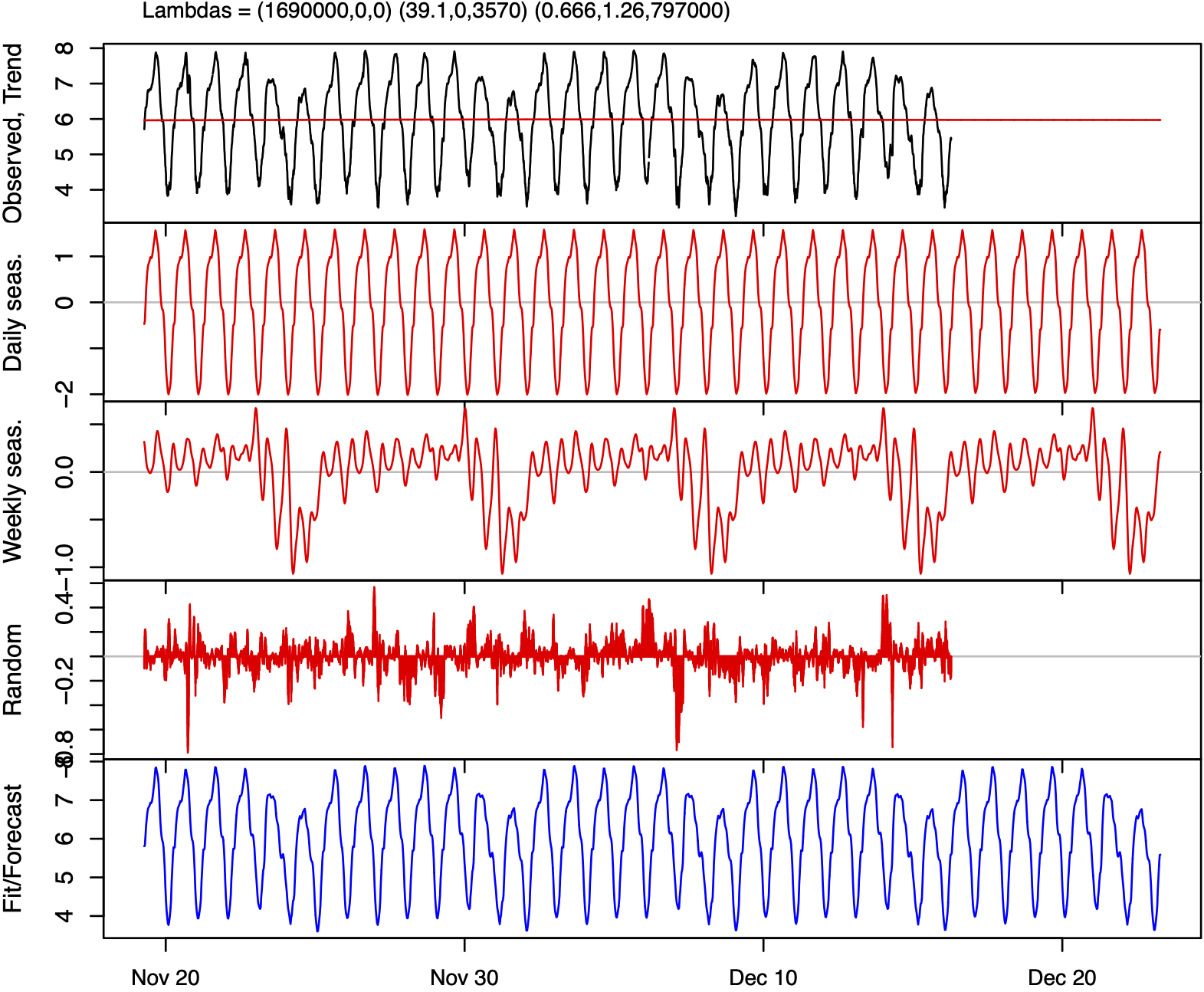
Figure 16: STR decomposition of the log transformed training data and the forecasts for the traffic flow data.

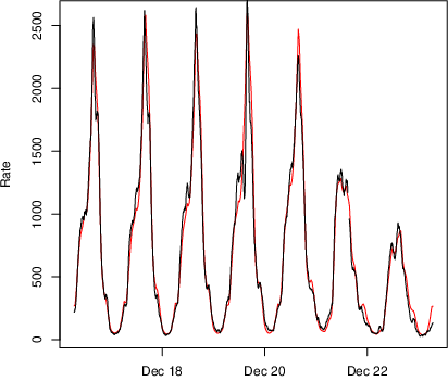
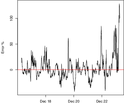
Figure 17: Left: forecast (red) and the test data (black); Right: the prediction error over time for the traffic flow data.

3.8.4 Call arrival forecasting¹⁵¹

Forecasting of inbound call arrivals for call centres supports a number of key decisions primarily around staffing (Aksin, Armony, & Mehrotra, 2007). This typically involves matching staffing level requirements to service demand as summarised in Figure 18. To achieve service level objectives, an understanding of the call load is required in terms of the call arrivals (Gans, Koole, & Mandelbaum, 2003). As such, forecasting of future call volume or call arrival rates is an important part of call centre management.

Figure 18: The staffing decision process in call centres.

There are several properties to call arrival data. Depending on the level of aggregation and the frequency with which data is collected, e.g., hourly, call arrival data may exhibit intraday (within-day), intraweek, and intrayear multiple seasonal patterns (Avramidis, Deslauriers, & L’Ecuyer, 2004; L. Brown et al., 2005 and §2.3.5). In addition, arrival data may also exhibit interday and intraday dependencies, with different time periods within the same day, or across days within the same week, showing strong levels of autocorrelation (L. Brown et al., 2005; Shen & Huang, 2005; Tanir & Booth, 1999). Call arrivals may also be heteroscedastic with variance at least proportional to arrival counts (Taylor, 2008), and overdispersed under a Poisson assumption having variance per time period typically much larger than its expected value (Avramidis et al., 2004; Jongbloed & Koole, 2001; Steckley, Henderson, & Mehrotra, 2005). These properties have implications for various approaches to modelling and forecasting call arrivals.

The first family of methods are time series methods requiring no distributional assumptions. Early studies employed auto regressive moving average (ARMA; see §2.3.4) models (Andrews & Cunningham, 1995; Antipov & Meade, 2002; Tandberg, Easom, & Qualls, 1995; Xu, 1999), exponential smoothing (Bianchi, Jarrett, & Hanumara, 1993, 1998 see §2.3.1), fast Fourier transforms (Lewis, Herbert, & Bell, 2003), and regression (Tych, Pedregal, Young, & Davies, 2002 see §2.3.2). The first methods capable of capturing multiple seasonality were evaluated by (Taylor, 2008) and included double seasonal exponential smoothing (James W Taylor, 2003b) and multiplicative double seasonal ARMA (SARMA). Since then several advanced time series methods have been developed and evaluated (De Livera et al., 2011; Taylor, 2010; James W Taylor & Snyder, 2012), including artificial neural networks (M. Li et al., 2011; Millán–Ruiz & Hidalgo, 2013; Pacheco, Millán-Ruiz, & Vélez, 2009) and models for density forecasting (James W Taylor, 2012).

Another family of models relies on the assumption of a time-inhomogeneous Poisson process adopting fixed (L. Brown et al., 2005; Jongbloed & Koole, 2001; Shen & Huang, 2008a; James W Taylor, 2012) and mixed modelling (Aldor-Noiman, Feigin, & Mandelbaum, 2009; Avramidis et al., 2004; Ibrahim & L’Ecuyer, 2013) approaches to account for the overdispersed nature of the data, and in some cases, interday and intraday dependence.

The works by Weinberg, Brown, & Stroud (2007) and Soyer & Tarimcilar (2008) model call volumes from a Bayesian point of view. Other Bayesian inspired approaches have been adopted mainly for estimating various model parameters, but also allowing for intraday updates of forecasts (Aktekin & Soyer, 2011; Landon, Ruggeri, Soyer, & Tarimcilar, 2010).

A further class of approach addresses the dimensionality challenge related to high frequency call data using Singular Value Decomposition (SVD). Shen & Huang (2005) and Shen & Huang (2008a) use the same technique to achieve dimensionality reduction of arrival data, and to create a forecasting model that provides both interday forecasts of call volume, and an intraday updating mechanism. Several further studies have extended the basic SVD approach to realise further modelling innovations, for example, to forecast call arrival rate profiles and generate smooth arrival rate curves (Shen, 2009; Shen & Huang, 2008b; Shen, Huang, & Lee, 2007). A more comprehensive coverage of different forecasting approaches for call arrival rate and volume can be found in a recent review paper by Ibrahim, Ye, L’Ecuyer, & Shen (2016).

3.8.5 Elections forecasting¹⁵²

With the exception of weather forecasts, there are few forecasts which have as much public exposure as election forecasts. They are frequently published by mass media, with their number and disclosure reaching a frenzy as the Election Day approaches. This explains the significant amount of methods, approaches and procedures proposed and the paramount role these forecasts play in shaping people’s confidence in (soft/social) methods of forecasting.

The problem escalates because, regardless whether the goal of the election forecast is an attempt to ascertain the winner in two-choice elections (e.g., a referendum or a Presidential election) or to reach estimates within the margins of error in Parliamentary systems, the knowledge of the forecasts influences electors’ choices (Pavı́a et al., 2019). Election forecasts not only affect voters but also political parties, campaign organizations and (international) investors, who are also watchful of their evolution.

Scientific approaches to election forecasting include polls, information (stock) markets and statistical models. They can also be sorted by when they are performed; and new methods, such as social media surveillance (see also §2.9.3), are also emerging (Ceron, Curini, & Iacus, 2016; Huberty, 2015). Probabilistic (representative) polls are the most commonly used instrument to gauge public opinions. The progressive higher impact of non-sampling errors (coverage issues, non-response bias, measurement error: Biemer, 2010) is, however, severely testing this approach. Despite this, as Kennedy, Wojcik, & Lazer (2017) show in a recent study covering 86 countries and more than 500 elections, polls are still powerful and robust predictors of election outcomes after adjustments (see also Jennings, Lewis-Beck, & Wlezien, 2020). The increasing need of post-sampling adjustments of probabilistic samples has led to a resurgence of interest in non-probabilistic polls (Elliott & Valliant, 2017; Pavı́a & Larraz, 2012; Wang et al., 2015), abandoned in favour of probabilistic sampling in 1936, when Gallup forecasted Roosevelt’s triumph over Landon using a small representative sample despite Literacy Digest failing to do so with a sample of near 2.5 million responses (Squire, 1988).

A person knows far more than just her/his voting intention (Rothschild, 2009) and when s/he makes a bet, the rationality of her/his prediction is reinforced because s/he wants to win. Expectation polls try to exloit the first issue (Graefe, 2014), while prediction markets, as efficient aggregators of information, exploit both these issues to yield election forecasts (see also §2.6.4 and §2.11.4). Several studies have proven the performance of these approaches (Berg, Nelson, & Rietz, 2008; Erikson & Wlezien, 2012; Williams & Reade, 2016; Wolfers & Zitzewitz, 2004), even studying their links with opinion polls (Brown, Reade, & Vaughan Williams, 2019). Practice has also developed econometric models (Fair, 1978) that exploit structural information available months before the election (e.g., the evolution of the economy or the incumbent popularity). Lewis-Beck has had great success in publishing dozens of papers using this approach (see, e.g., Lewis-Beck, 2005).

Special mention also goes to Election-Day forecasting strategies, which have been systematically commissioned since the 1950s (Mitofsky, 1991). Exit (and entrance) polls (Klofstad & Bishin, 2012; Pavı́a, 2010), quick-counts (Pavı́a-Miralles & Larraz-Iribas, 2008), and statistical models (Bernardo, 1984; Moshman, 1964; Pavı́a-Miralles, 2005) have been used to anticipate outcomes on Election Day. Some of these strategies (mainly random quick-counts) can be also employed as auditing tools to disclose manipulation and fraud in weak democracies (Scheuren & Alvey, 2008).

3.8.6 Sports forecasting¹⁵³

Forecasting is inherent to sport. Strategies employed by participants in sporting contests rely on forecasts, and the decision by promoters to promote, and consumers to attend such events are conditioned on forecasts: predictions of how interesting the event will be. First in this section, we look at forecast competitions in sport, and following this we consider the role forecasts play in sporting outcomes.

Forecast competitions are common; see §2.12.7. Sport provides a range of forecast competitions, perhaps most notably the competition between bookmakers and their customers – betting. A bet is a contingent contract, a contract whose payout is conditional on specified future events occurring. Bets occur fundamentally because two agents disagree about the likelihood of that event occurring, and hence it is a forecast.

Bookmakers have been extensively analysed as forecasters; Forrest, Goddard, & Simmons (2005) evaluated biases in the forecasts implied by bookmaker odds over a period where the betting industry became more competitive, and found that relative to expert forecasts, bookmaker forecasts improved.

With the internet age, prediction markets have emerged, financial exchanges where willing participants can buy and sell contingent contracts. In theory, such decentralised market structures ought to provide the most efficient prices and hence efficient forecasts (Nordhaus, 1987). A range of papers have tested this in the sporting context (Angelini & De Angelis, 2019; Croxson & Reade, 2014; Gil & Levitt, 2007), with conclusions tending towards a lack of efficiency.

judgmental forecasts by experts are commonplace too (see also §2.11); traditionally in newspapers, but more recently on television and online. Reade, Singleton, & Brown (2020) evaluate forecasts of scorelines from two such experts against bookmaker prices, a statistical model, and the forecasts from users of an online forecasting competition. Singleton, Reade, & Brown (2019) find that when forecasters in the same competition revise their forecasts, their forecast performance worsens. This forecasting competition is also analysed by Butler, Butler, & Eakins (2020) and Reade et al. (2020).

Sport is a spectacle, and its commercial success is conditioned on this fact. Hundreds of millions of people globally watch events like the Olympics and the FIFA World Cup – but such interest is conditioned on anticipation, a forecast that something interesting will happen. A superstar is going to be performing, the match will be a close encounter, or it will matter a lot for a bigger outcome (the championship, say). These are the central tenets of sport economics back to Neale (1964) and Rottenberg (1956), most fundamentally the ‘uncertainty of outcome hypothesis’. A multitude of sport attendance prediction studies investigate this (see, for example, Hart, Hutton, & Sharot, 1975; Coates & Humphreys, 2010; Forrest & Simmons, 2006; Ours, 2021; Sacheti, Gregory-Smith, & Paton, 2014), and Van Reeth (2019) considers this for forecasting TV audiences for the Tour de France.

Cities and countries bid to host large events like the World Cup based on forecasts regarding the impact of hosting such events. Forecasts that are often inflated for political reasons (Baade & Matheson, 2016). Equally, franchise-based sports like many North American sports attract forecasts regarding the impact of a team locating in a city, usually resulting in public subsidies for the construction of venues for teams to play at (Coates & Humphreys, 1999). Governments invest in sporting development, primarily to achieve better performances at global events, most notably the Olympics (Bernard & Busse, 2004).

Many sporting events themselves rely on forecasts to function; high jumpers predict what height they will be able to jump over, and free diving contestants must state the depth they will dive to. Less formally, teams will set themselves goals: to win matches, to win competitions, to avoid the ‘wooden spoon’. Here, forecast outcomes are influenced by the teams, and competitors, taking part in competitions and, as such, are perhaps less commonly thought of as genuine forecasts. Important works predicting outcomes range from Dixon & Coles (1997) in soccer, to Kovalchik & Reid (2019) for tennis, while the increasing abundance of data means that machine learning and deep learning methods are beginning to dominate the landscape. See, for example, Maymin (2019) and Hubáček, Šourek, & Železnỳ (2019) for basketball, and Mulholland & Jensen (2019) for NFL.

3.8.7 Forecasting for megaprojects¹⁵⁴

Megaprojects are significant activities characterised by a multi-organisation structure, which produces highly visible infrastructure or asset with very crucial social impacts (Aaltonen, 2011). Megaprojects are complex, require huge capital investment, several stakeholders are identified and, usually a vast number of communities and the public are the receivers of the project’s benefits. There is a need megaprojects especially those that deliver social and economic goods and create economic growth (Flyvbjerg, Bruzelius, & Rothengatter, 2003). Typical features of megaprojects include some or all the following: (i) delivering a substantial piece of physical infrastructure with a life expectancy that spans across decades, (ii) main contractor or group of contractors are privately owned and financed, and (iii) the contractor could retain an ownership stake in the project and the client is often a government or public sector organisation (Sanderson, 2012).

However, megaprojects are heavily laced with extreme human and technical complexities making their delivery and implementation difficult and often unsuccessful (Merrow, McDonnell, & Arguden, 1988; The RFE Working Group Report, 2015). This is largely due to the challenge of managing megaprojects including extreme complexity, increased risk, tight budget and deadlines, lofty ideals (Fiori & Kovaka, 2005). Due to the possibility and consequences of megaproject failure (Mišić & Radujković, 2015), forecasting the outcomes of megaprojects is becoming of growing importance. In particular, it is crucial to identify and assess the risks and uncertainties as well as other factors that contribute to disappointing outcomes of megaprojects in order to mitigate them (Flyvbjerg et al., 2003; Miller & Lessard, 2007).

Literature review in forecasting in megaprojects are scarce. However, there are a few themes that have emerged in the extant literature as characteristics of megaprojects that should be skilfully managed to provide a guideline for the successful planning and construction of megaprojects (Fiori & Kovaka, 2005; Flyvbjerg, 2007; Sanderson, 2012). Turner & Zolin (2012) even claim that we cannot even properly define what success is. They argue that we need to reliable scales in order to predict multiple perspectives by multiple stakeholders over multiple time frames — so definitely a very difficult long term problem. This could be done via a set of leading performance indicators that will enable managers of Megaprojects to forecast during project execution how various stakeholders will perceive success months or even years into the operation. At the very early stages of a project’s lifecycle, a number of decisions must been taken and are of a great importance for the performance and successful deliverables/outcomes. Flyvbjerg (2007) stress the importance of the front-end considerations particularly for Megaprojects Failure to account for unforeseen events frequently lead to cost overruns.

Litsiou et al. (2019) suggest that forecasting the success of megaprojects is particularly a challenging and critical task due to the characteristics of such projects. Megaproject stakeholders typically implement impact assessments and/or cost benefit Analysis tools (Litsiou et al., 2019). As Makridakis, Hogarth, & Gaba (2010) suggested, judgmental forecasting is suitable where quantitative data is limited, and the level of uncertainty is very high; elements that we find in megaprojects. By comparing the performance of three judgmental methods, unaided judgment, semi-structured analogies (sSA), and interaction groups (IG), used by a group of 69 semi-experts, Litsiou et al. (2019) found that, the use of sSA outperforms unaided judgment in forecasting performance (see also §2.11.4). The difference is amplified further when pooling of analogies through IG is introduced.

3.8.8 Competing products¹⁵⁵

Competition among products or technologies affects prediction due to local systematic deviations and saturating effects related to policies, and evolving interactions. The corresponding sales time series must be jointly modelled including the time varying reciprocal influence. Following the guidelines in subsection §2.3.20, some examples are reported below.

Based on IMS-Health quarterly number of cimetidine and ranitidine packages sold in Italy, the CRCD model (Guseo & Mortarino, 2012) was tested to evaluate a diachronic competition that produced substitution. Cimetidine is a histamine antagonist that inhibits the production of stomach acid and was introduced by Smith, Kline & French in 1976. Ranitidine is an alternative active principle introduced by Glaxo in 1981 and was found to have far-improved tolerability and a longer-lasting action. The main effect in delayed competition is that the first compound spread fast but was suddenly outperformed by the new one principle that modified its stand-alone regime. Guseo & Mortarino (2012) give some statistical and forecasting comparisons with the restricted Krishnan-Bass-Kummar Diachronic model (KBKD) by Krishnan et al. (2000). Previous results were improved with the UCRCD model in Guseo & Mortarino (2014) by considering a decomposition of word-of-mouth (WOM) effects in two parts: within-brand and cross-brand contributions. The new active compound exploited a large cross-brand WOM and a positive within-brand effect. After the start of competition, cimetidine experienced a negative WOM effect from its own adopters and benefited from the increase of the category’s market potential driven by the antagonist. Forecasting is more realistic with the UCRCD approach and it avoids mistakes in long-term prediction.

Restricted and unrestricted UCRCD models were applied in Germany by Guidolin & Guseo (2016) to the competition between nuclear power technologies and renewable energy technologies (wind and solar; see also §3.4.5, §3.4.6 and §3.4.8) in electricity production. Due to the ‘Energiewende’ policy started around 2000, the substitution effect, induced by competition, is confirmed by the electricity production data provided by BP¹⁵⁶. An advance is proposed in Furlan, Mortarino, & Zahangir (2020) with three competitors (nuclear power, wind, and solar technologies) and exogenous control functions obtaining direct inferences that provide a deeper analysis and forecasting improvements in energy transition context.

Previous mentioned intersections between Lotka-Volterra approach and diffusion of innovations competition models suggested a more modulated access to the residual carrying capacity. The Lotka-Volterra with churn model (LVch) by Guidolin & Guseo (2015) represents ‘churn effects’ preserving within and cross-brand effects in a synchronic context.

An application of LVch model is discussed with reference to the competition/substitution between compact cassettes and compact discs for pre-recorded music in the US market. Obtained results of LVch outperform restricted and unrestricted UCRCD analyses. In this context the residual market is not perfectly accessible to both competitors and this fact, combined with WOM components, allows for better interpretation and forecasting especially in medium and long-term horizons.

A further application of the LVch model, Lotka-Volterra with asymmetric churn (LVac), is proposed in Guidolin & Guseo (2020). It is based on a statistical reduction: The late entrant behaves as a standard Bass (1969) model that modifies the dynamics and the evolution of the first entrant in a partially overlapped market. The case study is offered by a special form of competition where the iPhone produced an inverse cannibalisation of the iPad. The former suffered a local negative interaction with some benefits: A long-lasting life cycle and a larger market size induced by the iPad.

A limitation in models for diachronic competition relates to high number of rivals, implying complex parametric representations with respect to the observed information. A second limitation, but also an opportunity, is the conditional nature of forecasting if the processes partially depend upon exogenous control functions (new policy regulations, new radical innovations, regular and promotional prices, etc.). These tools may be used to simulate the effect of strategic interventions, but a lack of knowledge of such future policies may affect prediction.

3.8.9 Forecasting under data integrity attacks¹⁵⁷

Data integrity attacks, where unauthorized parties access protected or confidential data and inject false information using various attack templates such as ramping, scaling, random attacks, pulse and smooth-curve, has become a major concern in data integrity control in forecasting (Giani et al., 2013; Singer & Friedman, 2014; Sridhar & Govindarasu, 2014; Yue, 2017).

Several previous studies have given attention in anomaly detection pre-processing step in forecasting workflow with varying degree of emphasis. However, according to Yue (2017), the detection of data integrity attacks is very challenging as such attacks are done by highly skilled adversaries in a coordinated manner without notable variations in the historical data patterns (Liang, He, & Chen, 2019). These attacks can cause over-forecasts that demand unnecessary expenses for the upgrade and maintenance, and can eventually lead to poor planning and business decisions (Luo et al., 2018a; Jian Luo et al., 2018b; Wu, Yu, Cui, & Lu, 2020).

Short-term load forecasting (see §3.4.3) is one major field that are vulnerable to malicious data integrity attacks as many power industry functions such as economic dispatch, unit commitment and automatic generation control heavily depend on accurate load forecasts (Liang et al., 2019). The cyberattack on U.S. power grid in 2018 is one such major incident related to the topic. According to the study conducted by Luo et al. (2018a), the widely used load forecasting models fail to produce reliable load forecast in the presence of such large malicious data integrity attacks. A submission to the Global Energy Forecasting Competition 2014 (GEFCom2014) incorporated an anomaly detection pre-processing step with a fixed anomalous threshold to their load forecasting framework (Xie & Hong, 2016). The method was later improved by Luo et al. (2018c) by replacing the fixed threshold with a data driven anomalous threshold. Sridhar & Govindarasu (2014) also proposed a general framework to detect scaling and ramp attacks in power systems. Akouemo & Povinelli (2016) investigated the impact towards the gas load forecasting using hybrid approach based on Bayesian maximum likelihood classifier and a forecasting model. In contrast to the previous model based attempts, Yue, Hong, & Wang (2019) proposed a descriptive analytic-based approach to detect cyberattacks including long anomalous sub-sequences (see §2.2.3), that are difficult to detect by the conventional anomaly detection methods.

The problem of data integrity attacks is not limited to load forecasting. Forecasting fields such as elections forecasting (see §3.8.5), retail forecasting (see §3.2.4), airline flight demand forecasting (see §3.8.2) and stock price forecasting §3.3.13) are also vulnerable to data integrity attacks (Luo et al., 2018a; Seaman, 2018). For instant, Wu et al. (2020) explored the vulnerability of traffic modelling and forecasting in the presence of data integrity attacks with the aim of providing useful guidance for constrained network resource planning and scheduling.

However, despite of the increasing attention toward the topic, advancements in cyberattacks on critical infrastructure raise further data challenges. Fooling existing anomaly detection algorithms via novel cyberattack templates is one such major concern. In response to the above concern, Liang et al. (2019) proposed a data poisoning algorithm that can fool existing load forecasting approaches with anomaly detection component while demanding further investigation into advanced anomaly detection methods. Further, adversaries can also manipulate other related input data without damaging the target data series. Therefore, further research similar to (Sobhani et al., 2020) are required to handle such data challenges.

3.8.10 The forecastability of agricultural time series¹⁵⁸

The forecasting of agricultural time series falls under the broader group of forecasting commodities, of which agricultural and related products are a critical subset. While there has been considerable work in the econometrics and forecasting literature on common factor models in general there is surprisingly little work so far on the application of such models for commodities and agricultural time series – and this is so given that there is considerable literature in the linkage between energy and commodities, including agricultural products, their prices and futures prices, their returns and volatilities. Furthermore, a significant number of papers is fairly recent which indicates that there are many open avenues of future research on these topics, and in particular for applied forecasting. The literature on the latter connection can consider many different aspects in modelling as we illustrate below. We can identify two literature strands, a much larger one on the various connections of energy with commodities and the agricultural sector (and in this strand we include forecasting agricultural series) and a smaller one that explores the issue of common factors.

An early reference of the impact of energy on the agricultural sector is Tewari (1990) and then after a decade we find Gohin & Chantret (2010) on the long-run impact of energy prices on global agricultural markets. Byrne, Fazio, & Fiess (2013) is an early reference for co-movement of commodity prices followed by Daskalaki, Kostakis, & Skiadopoulos (2014) on common factors of commodity future returns and then a very recent paper from Alquist, Bhattarai, & Coibion (2020) who link global economic activity with commodity price co-movement. The impact of energy shocks on US agricultural productivity was investigated by S. L. Wang & McPhail (2014) while Koirala, Mishra, D’Antoni, & Mehlhorn (2015) explore the non-linear correlations of energy and agricultural prices with Albulescu, Tiwari, & Ji (2020) exploring the latter issue further, the last two papers using copulas. Xiong, Li, Bao, Hu, & Zhang (2015) is an early reference of forecasting agricultural commodity prices while Kyriazi et al. (2019), Jue Wang et al. (2019), and Jianping Li et al. (2020) consider three novel and completely different approaches on forecasting agricultural prices and agricultural futures returns. López Cabrera & Schulz (2016) explore volatility linkages between energy and agricultural commodity prices and then Tian, Yang, & Chen (2017) start a mini-stream on volatility forecasting on agricultural series followed among others by the work of Luo, Klein, Ji, & Hou (2019) and of Degiannakis, Filis, Klein, & Walther (2020). Nicola, De Pace, & Hernandez (2016) examine the co-movement of energy and agricultural returns while Kagraoka (2016) and Lübbers & Posch (2016) examine common factors in commodity prices. Wei Su, Wang, Tao, & Oana-Ramona (2019) and Pal & Mitra (2019) both investigate the linkages of crude oil and agricultural prices. Finally, Tiwari, Nasreen, Shahbaz, & Hammoudeh (2020) examine the time-frequency causality between various commodities, including agricultural and metals.

There is clearly room for a number of applications in the context of this recent research, such along the lines of further identifying and then using common factors in constructing forecasting models, exploring the impact of the COVID-19 crisis in agricultural production or that of climate changes on agricultural prices.

3.8.11 Forecasting in the food and beverage industry¹⁵⁹

Reducing the ecological impact and waste, and increasing the efficiency of the food and beverage industry are currently major worldwide issues. To this direction, efficient and sustainable management of perishable food and the control of the beverage quality is of paramount importance. A particular focus on this topic is placed on supply chain forecasting (see §3.2.2), with advanced monitoring technologies able to track the events impacting and affecting the food and beverage processes (La Scalia, Micale, Miglietta, & Toma, 2019). Such technologies are typically deployed inside manufacturing plants, yielding to Industry 4.0 solutions (Ojo, Shah, Coutroubis, Jiménez, & Ocana, 2018) that are enabled by state-of-the-art forecasting applications in smart factories. The transition from plain agriculture techniques to smart solutions for food processing is a trend that fosters emerging forecasting data-driven solutions in many parts of the world, with special attention to the sustainability aspects (Zailani, Jeyaraman, Vengadasan, & Premkumar, 2012).

Various forecasting approaches have been successfully applied in the context of the food and beverage industry, from Monte Carlo simulations based on a shelf-life model (La Scalia et al., 2019), to association rule mining (see §2.9.2) applied to sensor-based equipment monitoring measurements (Apiletti & Pastor, 2020), multi-objective mathematical models for perishable supply chain configurations, forecasting costs, delivery time, and emissions (C.-N. Wang et al., 2021), and intelligent agent technologies for network optimisation in the food and beverage logistics management (Mangina & Vlachos, 2005).

We now focus on the case of forecasting the quality of beverages, and particularly coffee. Espresso coffee is among the most popular beverages, and its quality is one of the most discussed and investigated issues. Besides human-expert panels, electronic noses, and chemical techniques, forecasting the quality of espresso by means of data-driven approaches, such as association rule mining, is an emerging research topic (Apiletti & Pastor, 2020; Apiletti et al., 2020; Kittichotsatsawat, Jangkrajarng, & Tippayawong, 2021).

The forecasting model of the espresso quality is built from a real-world dataset of espresso brewing by professional coffee-making machines. Coffee ground size, coffee ground amount, and water pressure have been selected among the most influential external variables. The ground-truth quality evaluation has been performed for each shot of coffee based on three well-known quality variables selected by domain experts and measured by specific sensors: the extraction time, the average flow rate, and the espresso volume. An exhaustive set of more than a thousand coffees has been produced to train a model able to forecast the effect of non-optimal values on the espresso quality.

For each variable considered, different categorical values are considered: ground size can be coarse, optimal, or fine; ground amount can be high, optimal, or low; brewing water pressure can be high, optimal, or low. The experimental setting of categorical variables enables the application of association rule mining (see §2.9.2), a powerful data-driven exhaustive and explainable approach (Han et al., 2011; Tan et al., 2005), successfully exploited in different application contexts (Acquaviva et al., 2015; Di Corso et al., 2018).

Several interesting findings emerged. If the water pressure is low, the amount of coffee ground is too high, and the grinding is fine, then we can forecast with confidence a low-quality coffee due to excessive percolation time. If the amount of coffee ground is low, the ground is coarse, and the pressure is high, then we can forecast a low-quality coffee due to excessive flow rate. Furthermore, the coarseness of coffee ground generates an excessive flow rate forecast, despite the optimal values of dosage and pressure, with very high confidence.

3.8.12 Dealing with logistic forecasts in practice¹⁶⁰

The forecaster faces three major difficulties when using the logistic equation (S curve); see also §2.3.19. A first dilemma is whether he or she should fit an S curve to the cumulative number or to the number per unit of time. Here the forecaster must exercise wise judgment. What is the “species” and what is the niche that is being filled? To the frustration of business people there is no universal answer. When forecasting the sales of a new product it is often clear that one should fit the cumulative sales because the product’s market niche is expected to eventually fill up. But if we are dealing with something that is going to stay with us for a long time (for example, the Internet or a smoking habit), then one should not fit cumulative numbers. At times this distinction may not be so obvious. For example, when COVID-19 first appeared many people (often amateurs) began fitting S curves to the cumulative number of infections (for other attempts on forecasting COVID-19, see §3.6.2). Some of them were rewarded because indeed the diffusion of the virus in some countries behaved accordingly (Debecker & Modis, 1994). But many were frustrated and tried to “fix” the logistic equation by introducing more parameters, or simply gave up on trying to use logistics with COVID 19. And yet, many cases (e.g., the US) can be illuminated by logistic fits but on the daily number of infections, not on the cumulative number. As of August 1, 2020, leaving out the three eastern states that had gotten things under control, the rest of the US displayed two classic S curve steps followed by plateaus (see Figure 19). The two plateaus reflect the number of infections that American society was willing to tolerate at the time, as the price to pay for not applying measures to restrict the virus diffusion.

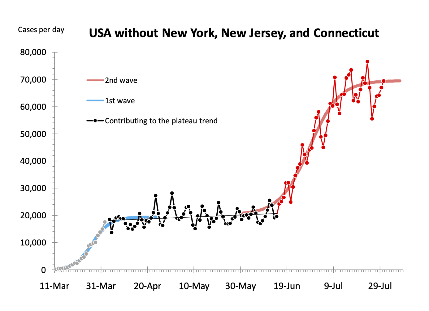
Figure 19: Two logistic-growth steps during the early diffusion of COVID-19 in America (March to July, 2020).

The second difficulty in using the logistic equation has to do with its ability to predict from relatively early measurements the final ceiling. The crucial question is how early can the final ceiling be determined and with what accuracy. Some people claim that before the midpoint no determination of a final level is trustworthy (Marinakis & Walsh, 2021). Forecasters usually abstain from assigning quantitative uncertainties on the parameters of their S curve forecasts mostly because there is no theory behind it. However, there is a unique study by Debecker & Modis (2021) that quantifies the uncertainties on the parameters determined by logistic fits. The study was based on 35,000 S curve fits on simulated data, smeared by random noise and covering a variety of conditions. The fits were carried out via a \(\chi^2\) minimisation technique. The study produced lookup tables and graphs for determining the uncertainties expected on the three parameters of the logistic equation as a function of the range of the S curve populated by data, the error per data point, and the confidence level required.

But a somewhat subjective argument can help us establish an upper limit to the expected final ceiling of a natural-growth process that grows along an S curve. During the very early stages an S curve is identical to an exponential curve. In order to be able to discern an S curve the growth process must proceed to the level where the pattern unambiguously differs from a simple exponential (T. Modis, 2013a). Let us try to see at what time a logistic function deviates from an exponential in a significant way (see Figure 20). Table 2 quantifies the deviation between the logistic and the corresponding exponential pattern as a fraction of the logistic’s level of completion. By “corresponding” exponential I mean the limit of \(X(t)\) as \(t \rightarrow -\infty\). \[X(t) = \frac{M}{1 + e^{-\alpha(t-t_0)}}.\]

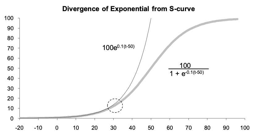
Figure 20: The construction of a theoretical S curve (gray line) and the exponential (thin black line) it reduces to as time goes backward. The big dotted circle points out the time when the deviation becomes important. The formulae used are shown in the graph.

In Table 2, we appreciate the size of the deviation between exponential and logistic patterns as a function of how much the logistic has been completed. Obviously beyond a certain point the difference becomes flagrant. When exactly this happens is subject to judgment. Table 2 helps decision makers quantitatively to make up their mind. Most will agree that at least 15% deviation between exponential and S-curve patterns is needed to make it clear that the two processes can no longer be confused. This happens when the logistic has reached a level of completion of about 13%. In other words, the future ceiling of an S curve that just begins deviating from an exponential pattern is at most 7 times the present level.

Table 2: The Deviation between exponential and logistic patterns as a function of how much the logistic has been completed.

Deviation	Completion level		Deviation	Completion level
11.1%	10.0%
12.2%	10.9%		36.8%	26.9%
13.5%	11.9%		40.7%	28.9%
15.0%	13.0%		44.9%	31.0%
16.5%	14.2%		49.7%	33.2%
18.3%	15.4%		54.9%	35.4%
20.2%	16.8%		60.7%	37.8%
22.3%	18.2%		67.0%	40.1%
24.7%	19.8%		74.1%	42.6%
27.3%	21.4%		81.9%	45.0%
30.1%	23.1%		90.5%	47.5%
33.3%	25.0%		100.0%	50.0%

A cruder more subjective rule-of-thumb estimation of an upper limit for an S curve can be obtained by exploiting the idea of infant mortality. For a natural-growth process to be describable by an S curve it must have grown beyond infant mortality. Based on the way trees grow we may define infant mortality — the period when a tree seedling is vulnerable to be stepped upon or be eaten by herbivore animals — as 5 to 10 percent of the final size. This puts an upper limit to the final ceiling of the S curve as 10 to 20 times its level at the end of infant mortality.

The third difficulty using the logistic equation comes from the fact that no matter what fitting program one uses, the fitted S curve will flatten toward a ceiling as early and as low as it is allowed by the constraints of the procedure. As a consequence fitting programs may yield logistic fits that are often biased toward a low ceiling. Bigger errors on the data points accentuate this bias by permitting larger margins for the determination of the S curve parameters. To compensate for this bias the user must explore several fits with different weights on the data points during the calculation of the \(\chi^2\). He or she should then favour the answer that gives the highest ceiling for the S curve (most often obtained by weighting more heavily the recent historical data points). Of course, this must be done with good justification; here again the forecaster must exercise wise judgment.

3.9 The future of forecasting practice¹⁶¹

Plus ça change, plus c’est la même chose.
Jean-Baptiste Karr (1849)

It would be a more straightforward task to make predictions about the future of forecasting practice if we had a better grasp of the present state of forecasting practice. For that matter, we lack even a common definition of forecasting practice. In a recent article, S. Makridakis et al. (2020) lamented the failure of truly notable advances in forecasting methodologies, systems, and processes during the past decades to convince many businesses to adopt systematic forecasting procedures, leaving a wide swath of commerce under the guidance of ad hoc judgment and intuition. At the other extreme, we see companies with implementations that combine state-of-the-art methodology with sophisticated accommodations of computing time and costs, as well as consideration of the requirements and capabilities of a diverse group of stakeholders (Yelland, Baz, & Serafini, 2019). So, it is not hyperbole to state that business forecasting practices are all over the place. What surely is hyperbole, however, are the ubiquitous claims of software providers about their products accurately forecasting sales, reducing costs, integrating functions, and elevating the bottom line (S. Makridakis et al., 2020; Sorensen, 2020). For this section, we grilled a dozen practitioners and thought leaders (“the Group”) about developments playing out in the next decade of forecasting practice, and have categorised their responses:

• Nature of forecasting challenges;

• Changes in the forecasting toolbox;

• Evolution in forecasting processes such as integration of planning functions;

• Expectations of forecasters; and

• Scepticism about real change.

Forecasting Challenges: Focusing on operations, the Group sees demand forecasting becoming ever more difficult due to product/channel proliferation, shorter lead times, shorter product histories, and spikes in major disruptions.

• Operational forecasts will have shorter forecast horizons to increase strategic agility required by business to compete, sustain, and survive.

• New models will need to incorporate supply-chain disruption. Demand chains will need to be restarted, shortening historical data sets and making traditional models less viable due to limited history.

• Lead times will decrease as companies see the problems in having distant suppliers. Longer lead times make accurate forecasting more difficult.

Forecasting Tool Box: Unsurprisingly, this category received most of the Group’s attention. All predict greater reliance on AI/ML for automating supply-and-demand planning tasks and for reconciling discrepancies in hierarchical forecasting. Longer-horizon causal forecasting models will be facilitated by big data, social media, and algorithmic improvements by quantum computing. Post-COVID, we will see a greater focus on risk management/mitigation. The Cloud will end the era of desktop solutions.

• Quantum computers will improve algorithms used in areas like financial forecasting (e.g., Monte Carlo simulations), and will change our thinking about forecasting and uncertainty.

• Although social media is a tool for “what’s trending now”, new models will be developed to use social-media data to predict longer-term behaviour. Step aside Brown (exponential smoothing) and Bass (diffusion).

• Greater automation of routine tasks (data loading, scrubbing, forecast generation and tuning, etc.) through AI/ML-powered workflow, configurable limits, and active alerts. More black box under the hood, but more clarity on the dashboard.

• Greater focus on risk management/mitigation through what-if scenarios, simulations, and probabilistic forecasting.

Forecasting Processes and Functional Integration: Systems will become more integrated, promoting greater collaboration across functional areas and coordination between forecast teams and those who rely upon them. Achieving supply-chain resilience will become as important as production efficiency, and new technology such as Alert and Root Cause Analysis systems will mitigate disruptions.

• S&OP will expand from its home in operations to more fully integrate with other functions such as finance and performance management, especially in larger multinationals.

• The pandemic has forced firms to consider upping supply-chain resilience. Firms are building in capacity, inventory, redundancy into operations—somewhat antithetical to the efficiency plays that forecasting brings to the table.

• Forecasting will be more closely tied to Alert and Root Cause Analysis systems, which identify breakdowns in processes/systems contributing to adverse events, and prevent their recurrence.

Expectations of Forecasters: Agreement was universal that the forecaster’s job description will broaden and become more demanding, but that technology will allow some redirection of effort from producing forecasts to communicating forecasting insights.

• The interest around disease models increases our awareness of the strengths and weaknesses of mathematical models. Forecasters may need to become more measured in their claims, or do more to resist their models being exploited.

• We will see a transformation from demand planner to demand analyst, requiring additional skill sets including advanced decision making, data and risk analysis, communication, and negotiation.

• Professional forecasters will be rare except in companies where this expertise is valued. Fewer students are now educated or interested in statistical modelling, and time is not generally available for training.

• Forecasters will learn the same lesson as optimisation folks in the 1990s and 2000s: the importance of understanding the application area—community intelligence.

Scepticism: Many were sceptical about the current enthusiasm for AI/ML methods; disappointed about the slow adoption of promising new methods into software systems and, in turn, by companies that use these systems; and pessimistic about the respect given to and influence of forecasters in the company’s decision making.

• While AI/ML are important additions to the forecaster’s toolbox, they will not automatically solve forecasting issues. Problems include data hunger, capacity brittleness, dubious input data, fickle trust by users (Kolassa, 2020c), and model bias.

• Practices in the next decade will look very similar to the present. Not that much has changed in the last decade, and academic developments are slow to be translated into practice.

• Politics, gaming, and the low priority given to forecasting are the prime drivers of practice, thus limiting interest in adopting new methodologies.

• None of the topical items (AI/ML, big data, demand sensing, new forecasting applications) will have much of an impact on forecasting practice. Forecasting departments hop from one trend to the other without making much progress towards better forecasting accuracy.

• Software companies will struggle, despite good offerings. Most companies do not want to invest in excellent forecasting engines; whatever came with their ERP system is “good enough”.

• Forecasting will continue to suffer from neglect by higher levels of management, particularly when forecasts are inconveniently contrary to the messages management hopes to convey.

Note finally that the COVID-19 pandemic has elevated practitioner concerns about disruptions to normal patterns as well as the fear of an increasingly volatile environment in which forecasts must be made. There are indications that companies will place more stress on judgmental scenarios, likely in conjunction with statistical/ML methods.

Bibliography

Aaltonen, K. (2011). Project stakeholder analysis as an environmental interpretation process. International Journal of Project Management, 29(2), 165–183. https://doi.org/10.1016/j.ijproman.2010.02.001

Abel, G. J. (2018). Non-zero trajectories for long-run net migration assumptions in global population projection models. Demographic Research, 38(54), 1635–1662.

AbouZahr, C., Savigny, D. de, Mikkelsen, L., Setel, P. W., Lozano, R., & Lopez, A. D. (2015). Towards universal civil registration and vital statistics systems: The time is now. The Lancet, 386(10001), 1407–1418. https://doi.org/10.1016/S0140-6736(15)60170-2

Abramson, B., & Finizza, A. (1991). Using belief networks to forecast oil prices. International Journal of Forecasting, 7(3), 299–315.

Abramson, B., & Finizza, A. (1995). Probabilistic forecasts from probabilistic models: A case study in the oil market. International Journal of Forecasting, 11(1), 63–72.

Acquaviva, A., Apiletti, D., Attanasio, A., Baralis, E., Castagnetti, F. B., Cerquitelli, T., … Patti, E. (2015). Enhancing energy awareness through the analysis of thermal energy consumption. In EDBT/icdt workshops (pp. 64–71).

Adams, W., & Michael, V. (1987). Short-term forecasting of passenger demand and some application in quantas. In AGIFORS symposium proc (Vol. 27).

Afanasyev, D. O., & Fedorova, E. A. (2019). On the impact of outlier filtering on the electricity price forecasting accuracy. Applied Energy, 236, 196–210. https://doi.org/10.1016/j.apenergy.2018.11.076

Agarwal, A., Dahleh, M., & Sarkar, T. (2019). A marketplace for data: An algorithmic solution. In Proceedings of the 2019 acm conference on economics and computation (pp. 701–726).

Agnolucci, P. (2009). Volatility in crude oil futures: A comparison of the predictive ability of GARCH and implied volatility models. Energy Economics, 31(2), 316–321.

Ahlburg, D. A., & Vaupel, J. W. (1990). Alternative projections of the U.S. population. Demography, 27(4), 639–652.

Ahmad, A., Javaid, N., Mateen, A., Awais, M., & Khan, Z. A. (2019). Short-Term load forecasting in smart grids: An intelligent modular approach. Energies, 12(1), 164. https://doi.org/10.3390/en12010164

Ahmad, A. S., Hassan, M. Y., Abdullah, M. P., Rahman, H. A., Hussin, F., Abdullah, H., & Saidur, R. (2014). A review on applications of ANN and SVM for building electrical energy consumption forecasting. Renewable and Sustainable Energy Reviews, 33, 102–109. https://doi.org/https://doi.org/10.1016/j.rser.2014.01.069

Ahmad, M. W., Mourshed, M., & Rezgui, Y. (2017). Trees vs neurons: Comparison between random forest and ANN for high-resolution prediction of building energy consumption. Energy and Buildings, 147, 77–89.

Aizenman, J., & Jinjarak, Y. (2013). Real Estate Valuation, Current Account and Credit Growth Patterns, Before and After the 2008-9 Crisis (Working paper series No. 19190). National Bureau of Economic Research.

Aı̈t-Sahalia, Y., Cacho-Diaz, J., & Laeven, R. J. A. (2015). Modeling financial contagion using mutually exciting jump processes. Journal of Financial Economics, 117(3), 585–606. https://doi.org/10.1016/j.jfineco.2015.03.002

Akouemo, H. N., & Povinelli, R. J. (2016). Probabilistic anomaly detection in natural gas time series data. International Journal of Forecasting, 32(3), 948–956.

Aksin, Z., Armony, M., & Mehrotra, V. (2007). The modern call center: A multi-disciplinary perspective on operations management research. Production and Operations Management, 16(6), 665–688.

Aktekin, T., & Soyer, R. (2011). Call center arrival modeling: A Bayesian state-space approach. Naval Research Logistics, 58(1), 28–42.

Al-Azzani, M. A., Davari, S., & England, T. J. (2020). An empirical investigation of forecasting methods for ambulance calls-a case study. Health Systems, 1–18.

Albulescu, C. T., Tiwari, A. K., & Ji, Q. (2020). Copula-based local dependence among energy, agriculture and metal commodities markets. Energy, 202, 117762. https://doi.org/10.1016/j.energy.2020.117762

Albuquerquemello, V. P. de, Medeiros, R. K. de, Nóbrega Besarria, C. da, & Maia, S. F. (2018). Forecasting crude oil price: Does exist an optimal econometric model? Energy, 155, 578–591.

Aldor-Noiman, S., Feigin, P. D., & Mandelbaum, A. (2009). Workload forecasting for a call center: Methodology and a case study. The Annals of Applied Statistics, 3(4), 1403–1447.

Alho, J. M., & Spencer, B. D. (2005). Statistical Demography and Forecasting. New York: Springer.

Al-Homoud, M. S. (2001). Computer-aided building energy analysis techniques. Building and Environment, 36(4), 421–433. https://doi.org/https://doi.org/10.1016/S0360-1323(00)00026-3

Ali, M. M., & Boylan, J. E. (2011). Feasibility principles for downstream demand inference in supply chains. Journal of the Operational Research Society, 62(3), 474–482. https://doi.org/10.1057/jors.2010.82

Ali, M. M., Boylan, J. E., & Syntetos, A. A. (2012). Forecast errors and inventory performance under forecast information sharing. International Journal of Forecasting, 28(4), 830–841. https://doi.org/10.1016/j.ijforecast.2010.08.003

Alizadeh, S., Brandt, M. W., & Diebold, F. X. (2002). Range-based estimation of stochastic volatility models. Journal of Finance, 57(3), 1047–1091. https://doi.org/10.1111/1540-6261.00454

Alkema, L., Raftery, A. E., Gerland, P., Clark, S. J., Pelletier, F., Buettner, T., & Heilig, G. K. (2011). Probabilistic projections of the total fertility rate for all countries. Demography, 48(3), 815–839. https://doi.org/10.1007/s13524-011-0040-5

Almeida, C., & Czado, C. (2012). Efficient Bayesian inference for stochastic time-varying copula models. Computational Statistics & Data Analysis, 56(6), 1511–1527.

Almeida Marques-Toledo, C. de, Degener, C. M., Vinhal, L., Coelho, G., Meira, W., Codeço, C. T., & Teixeira, M. M. (2017). Dengue prediction by the web: Tweets are a useful tool for estimating and forecasting dengue at country and city level. PLoS Neglected Tropical Diseases, 11(7), e0005729.

Almeida Pereira, G. A. de, & Veiga, Á. (2019). Periodic copula autoregressive model designed to multivariate streamflow time series modelling. Water Resources Management, 33(10), 3417–3431. https://doi.org/10.1007/s11269-019-02308-6

Aloui, R., Hammoudeh, S., & Nguyen, D. K. (2013). A time-varying copula approach to oil and stock market dependence: The case of transition economies. Energy Economics, 39, 208–221.

Alquist, R., Bhattarai, S., & Coibion, O. (2020). Commodity-price comovement and global economic activity. Journal of Monetary Economics, 112, 41–56. https://doi.org/10.1016/j.jmoneco.2019.02.004

Alquist, R., Kilian, L., & Vigfusson, R. J. (2013). Forecasting the price of oil. In Handbook of economic forecasting (Vol. 2, pp. 427–507). Elsevier.

Alvarado-Valencia, J. A., & Barrero, L. H. (2014). Reliance, trust and heuristics in judgmental forecasting. Computers in Human Behavior, 36, 102–113. https://doi.org/10.1016/j.chb.2014.03.047

Alvarez-Ramirez, J., Soriano, A., Cisneros, M., & Suarez, R. (2003). Symmetry/anti-symmetry phase transitions in crude oil markets. Physica A: Statistical Mechanics and its Applications, 322, 583–596.

Amarasinghe, A., Wichmann, O., Margolis, H. S., & Mahoney, R. T. (2010). Forecasting dengue vaccine demand in disease endemic and non-endemic countries. Human Vaccines, 6(9), 745–753.

Andersson, E., Kühlmann-Berenzon, S., Linde, A., Schiöler, L., Rubinova, S., & Frisén, M. (2008). Predictions by early indicators of the time and height of the peaks of yearly influenza outbreaks in sweden. Scandinavian Journal of Public Health, 36(5), 475–482. https://doi.org/10.1177/1403494808089566

Andrade, J. R., Filipe, J., Reis, M., & Bessa, R. J. (2017). Probabilistic price forecasting for day-ahead and intraday markets: Beyond the statistical model. Sustainability, 9(1990), 1–29.

Andrews, B. H., & Cunningham, S. M. (1995). LL bean improves call-center forecasting. Interfaces, 25(6), 1–13.

Andrews, R. L., Currim, I. S., Leeflang, P., & Lim, J. (2008). Estimating the SCAN* PRO model of store sales: HB, FM or just OLS? International Journal of Research in Marketing, 25(1), 22–33.

Ang, A., & Bekaert, G. (2002). Short rate nonlinearities and regime switches. Journal of Economic Dynamics & Control, 26(7), 1243–1274. https://doi.org/10.1016/S0165-1889(01)00042-2

Ang, A., Bekaert, G., & Wei, M. (2008). The term structure of real rates and expected inflation. The Journal of Finance, 63(2), 797–849. https://doi.org/10.1111/j.1540-6261.2008.01332.x

Angelini, G., & De Angelis, L. (2019). Efficiency of online football betting markets. International Journal of Forecasting, 35(2), 712–721.

Antipov, A., & Meade, N. (2002). Forecasting call frequency at a financial services call centre. Journal of the Operational Research Society, 53(9), 953–960.

Antonakakis, N., Chatziantoniou, I., Floros, C., & Gabauer, D. (2018). The dynamic connectedness of U.K. regional property returns. Urban Studies, 55(14), 3110–3134.

Apiletti, D., & Pastor, E. (2020). Correlating espresso quality with coffee-machine parameters by means of association rule mining. Electronics, 9(1), 100.

Apiletti, D., Pastor, E., Callà, R., & Baralis, E. (2020). Evaluating espresso coffee quality by means of time-series feature engineering. In EDBT/icdt workshops.

Armstrong, C. (2017). Omnichannel retailing and demand planning. The Journal of Business Forecasting, 35(4), 10–15.

Armstrong, J. S., & Collopy, F. (1998). Integration of statistical methods and judgment for time series forecasting: Principles from empirical research. In G. Wright & P. Goodwin (Eds.), Forecasting with judgment (pp. 269–293). New York: John Wiley & Sons Ltd.

Arnott, R. D., Beck, N., Kalesnik, V., & West, J. (2016). How can “smart beta” go horribly wrong? SSRN:3040949.

Aron, J., & Muellbauer, J. (2020). Measuring excess mortality: The case of England during the Covid-19 pandemic. https://www.oxfordmartin.ox.ac.uk/publications/measuring-excess-mortality-the-case-of-england-during-the-covid-19-pandemic/; Oxford: INET Oxford Working Paper.

Arora, S., Taylor, J. W., & Mak, H.-Y. (2020). Probabilistic forecasting of patient waiting times in an emergency department. arXiv:2006.00335.

Arrhenius, S. A. (1896). On the influence of carbonic acid in the air upon the temperature of the ground. London, Edinburgh, and Dublin Philosophical Magazine and Journal of Science (Fifth Series), 41, 237–275.

Artis, M., & Marcellino, M. (2001). Fiscal forecasting: The track record of the imf, oecd and ec. The Econometrics Journal, 4(1), S20–S36.

Arvan, M., Fahimnia, B., Reisi, M., & Siemsen, E. (2019). Integrating human judgement into quantitative forecasting methods: A review. Omega, 86, 237–252. https://doi.org/10.1016/j.omega.2018.07.012

Asai, M., & Brugal, I. (2013). Forecasting volatility via stock return, range, trading volume and spillover effects: The case of Brazil. North American Journal of Economics and Finance, 25, 202–213. https://doi.org/10.1016/j.najef.2012.06.005

Asimakopoulos, S., & Dix, A. (2013). Forecasting support systems technologies-in-practice: A model of adoption and use for product forecasting. International Journal of Forecasting, 29(2), 322–336. https://doi.org/http://dx.doi.org/10.1016/j.ijforecast.2012.11.004

Asimakopoulos, S., Paredes, J., & Warmedinger, T. (2020). Real-time fiscal forecasting using mixed-frequency data. The Scandinavian Journal of Economics, 122, 369–390.

Asness, C. S. (2016). INVITED editorial comment: The siren song of factor timing aka “smart beta timing” aka “style timing”. Journal of Portfolio Management, 42(5), 1–6. Journal Article. https://doi.org/10.3905/jpm.2016.42.5.001

Assmus, G. (1984). New product forecasting. Journal of Forecasting, 3(2), 121–138. https://doi.org/10.1002/for.3980030202

Athanasopoulos, G., Ahmed, R. A., & Hyndman, R. J. (2009). Hierarchical forecasts for Australian domestic tourism. International Journal of Forecasting, 25(1), 146–166. https://doi.org/https://doi.org/10.1016/j.ijforecast.2008.07.004

Athanasopoulos, G., Hyndman, R. J., Song, H., & Wu, D. C. (2011). The tourism forecasting competition. International Journal of Forecasting, 27(3), 822–844. https://doi.org/10.1016/j.ijforecast.2010.04.009

Austin, C., & Kusumoto, F. (2016). The application of big data in medicine: Current implications and future directions. Journal of Interventional Cardiac Electrophysiology, 47(1), 51–59.

Avramidis, A. N., Deslauriers, A., & L’Ecuyer, P. (2004). Modeling daily arrivals to a telephone call center. Management Science, 50(7), 896–908.

Azose, J. J., & Raftery, A. E. (2015). Bayesian probabilistic projection of international migration. Demography, 52(5), 1627–1650. https://doi.org/10.1007/s13524-015-0415-0

Azose, J. J., Ševčı́ková, H., & Raftery, A. E. (2016). Probabilistic population projections with migration uncertainty. Proceedings of the National Academy of Sciences of the United States of America, 113(23), 6460–6465. https://doi.org/10.1073/pnas.1606119113

Baade, R. A., & Matheson, V. A. (2016). Going for the Gold: The economics of the Olympics. Journal of Economic Perspectives, 30(2), 201–18.

Baardman, L., Levin, I., Perakis, G., & Singhvi, D. (2018). Leveraging comparables for new product sales forecasting. Production and Operations Management, 27(12), 2340–2343.

Babai, M. Z., Dallery, Y., Boubaker, S., & Kalai, R. (2019). A new method to forecast intermittent demand in the presence of inventory obsolescence. International Journal of Production Economics, 209, 30–41. https://doi.org/10.1016/j.ijpe.2018.01.026

Babai, M. Z., Syntetos, A., & Teunter, R. (2014). Intermittent demand forecasting: An empirical study on accuracy and the risk of obsolescence. International Journal of Production Economics, 157, 212–219.

Babu, A., Levine, A., Ooi, Y. H., Pedersen, L. H., & Stamelos, E. (2020). Trends everywhere. Journal of Investment Management, 18(1), 52–68. Journal Article.

Bacchetti, A., & Saccani, N. (2012). Spare parts classification and demand forecasting for stock control: Investigating the gap between research and practice. Omega, 40(6), 722–737. https://doi.org/10.1016/j.omega.2011.06.008

Bacha, H., & Meyer, W. (1992). A neural network architecture for load forecasting. In IJCNN international joint conference on neural networks (Vol. 2, pp. 442–447).

Baecke, P., De Baets, S., & Vanderheyden, K. (2017). Investigating the added value of integrating human judgement into statistical demand forecasting systems. International Journal of Production Economics, 191, 85–96. https://doi.org/10.1016/j.ijpe.2017.05.016

Baicker, K., Chandra, A., & Skinner, J. S. (2012). Saving money or just saving lives? Improving the productivity of US health care spending. Annual Review of Economics, 4(1), 33–56.

Baker, J. (2021). Maximizing forecast value added through machine learning and nudges. Foresight: The International Journal of Applied Forecasting, 60.

Baker, S. R., Bloom, N., & Davis, S. J. (2016). Measuring economic policy uncertainty. The Quarterly Journal of Economics, 131(4), 1593–1636.

Balbo, N., Billari, F. C., & Mills, M. (2013). Fertility in advanced societies: A review of research. European Journal of Population, 29(1), 1–38. https://doi.org/10.1007/s10680-012-9277-y

Bandara, K., Bergmeir, C., & Hewamalage, H. (2020a). LSTM-MSNet: leveraging forecasts on sets of related time series with multiple seasonal patterns. IEEE Transactions on Neural Networks and Learning Systems.

Bandara, K., Bergmeir, C., & Smyl, S. (2020b). Forecasting across time series databases using recurrent neural networks on groups of similar series: A clustering approach. Expert Systems with Applications, 140, 112896.

Bandyopadhyay, S. (2009). A dynamic model of cross-category competition: Theory, tests and applications. Journal of Retailing, 85(4), 468–479.

Bangwayo-Skeete, P. F., & Skeete, R. W. (2015). Can Google data improve the forecasting performance of tourist arrivals? Mixed-data sampling approach. Tourism Management, 46, 454–464. https://doi.org/10.1016/j.tourman.2014.07.014

Banks, J., Blundell, R., Oldfield, Z., & Smith, J. P. (2015). House price volatility and the housing ladder (Working paper series No. 21255). National Bureau of Economic Research.

Bannister, R. N., Chipilski, H. G., & Martinez-Alvarado, O. (2020). Techniques and challenges in the assimilation of atmospheric water observations for numerical weather prediction towards convective scales. Quarterly Journal of the Royal Meteorological Society, 146(726), 1–48.

Bansal, R., Tauchen, G., & Zhou, H. (2004). Regime shifts, risk premiums in the term structure, and the business cycle. Journal of Business & Economic Statistics, 22(4), 396–409. https://doi.org/10.1198/073500104000000398

Bansal, R., & Zhou, H. (2002). Term structure of interest rates with regime shifts. The Journal of Finance, 57(5), 1997–2043. https://doi.org/10.1111/0022-1082.00487

Banu, S., Hu, W., Hurst, C., & Tong, S. (2011). Dengue transmission in the asia-pacific region: Impact of climate change and socio-environmental factors. Tropical Medicine & International Health, 16(5), 598–607.

Bańbura, M., Giannone, D., & Reichlin, L. (2010). Large bayesian vector auto regressions. Journal of Applied Econometrics, 25(1), 71–92. https://doi.org/10.1002/jae.1137

Bao, Y., Lee, T.-H., & Saltoglu, B. (2007). Comparing density forecast models. Journal of Forecasting, 26(3), 203–225.

Baptista, M., Sankararaman, S., Medeiros, I. P. de, Nascimento, C., Prendinger, H., & Henriques, E. M. P. (2018). Forecasting fault events for predictive maintenance using data-driven techniques and ARMA modeling. Computers & Industrial Engineering, 115, 41–53. https://doi.org/10.1016/j.cie.2017.10.033

BarclayHedge. (2018). Survey: Majority of hedge fund pros use AI/Machine learning in investment strategies. https://www.barclayhedge.com/insider/barclayhedge-survey-majority-of-hedge-fund-pros-use-ai-machine-learning-in-investment-strategies.

Barnhart, C., & Cohn, A. (2004). Airline schedule planning: Accomplishments and opportunities. Manufacturing & Service Operations Management, 6(1), 3–22.

Barnhart, C., Fearing, D., & Vaze, V. (2014). Modeling passenger travel and delays in the national air transportation system. Operations Research, 62(3), 580–601.

Barnichon, R., & Garda, P. (2016). Forecasting unemployment across countries: The ins and outs. European Economic Review, 84, 165–183.

Barr, J. (2018). New – predictive scaling for EC2, powered by machine learning. https://aws.amazon.com/blogs/aws/new-predictive-scaling-for-ec2-powered-by-machine-learning.

Barroso, P. (2015). Momentum has its moments. Journal of Financial Economics, 116(1), 111–121. Journal Article. https://doi.org/10.1016/j.jfineco.2014.11.010

Bartelsman, E. J., Kurz, C. J., & Wolf, Z. (2011). Using Census Microdata to Forecast US Aggregate Productivity. Working Paper.

Bartelsman, E. J., & Wolf, Z. (2014). Forecasting aggregate productivity using information from firm-level data. Review of Economics and Statistics, 96(4), 745–755.

Bass, F. M. (1969). A new product growth model for consumer durables. Management Science, 15, 215–227.

Bass, F. M., Gordon, K., Ferguson, T. L., & Githens, M. L. (2001). DIRECTV: Forecasting diffusion of a new technology prior to product launch. INFORMS Journal on Applied Analytics, 31(3S), S82–S93. https://doi.org/10.1287/inte.31.3s.82.9677

Basu, S., Fernald, J. G., Oulton, N., & Srinivasan, S. (2003). The case of the missing productivity growth, or does information technology explain why productivity accelerated in the United States but not in the United Kingdom? NBER Macroeconomics Annual, 18, 9–63.

Bates, J. M., & Granger, C. W. J. (1969). The combination of forecasts. Journal of the Operational Research Society, 20(4), 451–468.

Baumeister, C., Guérin, P., & Kilian, L. (2015). Do high-frequency financial data help forecast oil prices? The MIDAS touch at work. International Journal of Forecasting, 31(2), 238–252.

Baumeister, C., & Kilian, L. (2015). Forecasting the real price of oil in a changing world: A forecast combination approach. Journal of Business & Economic Statistics, 33(3), 338–351.

Becker, R., Hurn, S., & Pavlov, V. (2008). Modelling spikes in electricity prices. The Economic Record, 83(263), 371–382. https://doi.org/10.1111/j.1475-4932.2007.00427.x

Beckmann, J., & Schussler, R. (2016). Forecasting exchange rates under parameter and model uncertainty. Journal of International Money and Finance, 60, 267–288.

Beckmann, M., & Bobkoski, F. (1958). Airline demand: An analysis of some frequency distributions. Naval Research Logistics Quarterly, 5(1), 43–51.

Bekaert, G., Hodrick, R. J., & Marshall, D. A. (2001). Peso problem explanations for term structure anomalies. Journal of Monetary Economics, 48(2), 241–270.

Bekiros, S., Cardani, R., Paccagnini, A., & Villa, S. (2016). Dealing with financial instability under a DSGE modeling approach with banking intermediation: A predictability analysis versus TVP-VARs. Journal of Financial Stability, 26(C), 216–227. https://doi.org/10.1016/j.jfs.2016.07.006

Bekiros, S. D., & Paccagnini, A. (2014). Bayesian forecasting with small and medium scale factor-augmented vector autoregressive DSGE models. Computational Statistics & Data Analysis, 71(C), 298–323.

Bekiros, S. D., & Paccagnini, A. (2015). Macroprudential Policy And Forecasting Using Hybrid DSGE Models With Financial Frictions And State Space Markov-Switching Tvp-Vars. Macroeconomic Dynamics, 19(7), 1565–1592.

Bekiros, S. D., & Paccagnini, A. (2016). Policy Oriented Macroeconomic Forecasting with Hybrid DGSE and Time Varying Parameter VAR Models. Journal of Forecasting, 35(7), 613–632.

Bekiros, S., & Paccagnini, A. (2015). Estimating point and density forecasts for the US economy with a factor-augmented vector autoregressive DSGE model. Studies in Nonlinear Dynamics & Econometrics, 19(2), 107–136.

Beliën, J., & Forcé, H. (2012). Supply chain management of blood products: A literature review. European Journal of Operational Research, 217(1), 1–16. https://doi.org/10.1016/j.ejor.2011.05.026

Benati, L. (2007). Drift and breaks in labor productivity. Journal of Economic Dynamics and Control, 31(8), 2847–2877.

Bender, J., Sun, X., Thomas, R., & Zdorovtsov, V. (2018). The promises and pitfalls of factor timing. Journal of Portfolio Management, 44(4), 79–92. Journal Article. https://doi.org/10.3905/jpm.2018.44.4.079

Bennell, J., & Sutcliffe, C. (2004). Black-Scholes versus artificial neural networks in pricing FTSE 100 options. Intelligent Systems in Accounting, Finance & Management, 12(4), 243–260. https://doi.org/10.1002/isaf.254

Berdugo, V., Chaussin, C., Dubus, L., Hebrail, G., & Leboucher, V. (2011). Analog method for collaborative very-short-term forecasting of powergeneration from photovoltaic systems. In Next generation data mining summit (pp. 1–5). Athens, Greece.

Berg, J. E., Nelson, F. D., & Rietz, T. A. (2008). Prediction market accuracy in the long run. International Journal of Forecasting, 24(2), 285–300. https://doi.org/10.1016/j.ijforecast.2008.03.007

Berger, J. O. (1985). Statistical decision theory and bayesian analysis. Springer.

Berkowitz, J. (2001). Testing density forecasts, with applications to risk management. Journal of Business & Economic Statistics, 19(4), 465–474. https://doi.org/10.1198/07350010152596718

Berlinski, D. (2009). The devil’s delusion: Atheism and its scientific pretensions. Basic Books.

Bernard, A. B., & Busse, M. R. (2004). Who wins the Olympic Games: Economic resources and medal totals. Review of Economics and Statistics, 86(1), 413–417.

Bernardo, J. M. (1984). Monitoring the 1982 spanish socialist victory: A bayesian analysis. Journal of the American Statistical Association, 79(387), 510–515. https://doi.org/10.1080/01621459.1984.10478077

Bernardo, J. M. (1994). Bayesian theory. Wiley.

Bernstein, R. (1995). Style investing. Book, New York: John Wiley & Sons.

Bessa, R. J., Miranda, V., Botterud, A., Zhou, Z., & Wang, J. (2012). Time-adaptive quantile-copula for wind power probabilistic forecasting. Renewable Energy, 40(1), 29–39.

Bessa, R. J., Möhrlen, C., Fundel, V., Siefert, M., Browell, J., Haglund El Gaidi, S., … Kariniotakis, G. (2017). Towards improved understanding of the applicability of uncertainty forecasts in the electric power industry. Energies, 10(9). https://doi.org/doi:10.3390/en10091402

Bianchi, L., Jarrett, J. E., & Hanumara, R. C. (1993). Forecasting incoming calls to telemarketing centers. The Journal of Business Forecasting, 12(2), 3.

Bianchi, L., Jarrett, J., & Hanumara, R. C. (1998). Improving forecasting for telemarketing centers by ARIMA modeling with intervention. International Journal of Forecasting, 14(4), 497–504.

Bielecki, T. R., & Rutkowski, M. (2013). Credit risk: Modeling, valuation and hedging. Springer Science & Business Media.

Biemer, P. P. (2010). Total survey error: Design, implementation, and evaluation. Public Opinion Quarterly, 74(5), 817–848. https://doi.org/10.1093/poq/nfq058

Bijak, J. (2010). Forecasting international migration in europe: A bayesian view. Springer, Dordrecht. https://doi.org/10.1007/978-90-481-8897-0

Bijak, J., & Czaika, M. (2020). Black swans and grey rhinos: Migration policy under uncertainty. Migration Policy Practice, X(4), 14–20.

Bijak, J., Disney, G., Findlay, A. M., Forster, J. J., Smith, P. W. F., & Wiśniowski, A. (2019). Assessing time series models for forecasting international migration: Lessons from the united kingdom. Journal of Forecasting, 38(6), 470–487. https://doi.org/10.1002/for.2576

Bijak, J., & Wiśniowski, A. (2010). Bayesian forecasting of immigration to selected european countries by using expert knowledge. Journal of the Royal Statistical Society. Series A, 173(4), 775–796.

Binder, C. C. (2017). Measuring uncertainty based on rounding: New method and application to inflation expectations. Journal of Monetary Economics, 90(C), 1–12.

Bjerknes, V. (1904). Das problem der wettervorhersage, betrachtet vom standpunkte der mechanik und der physik. Meteorologische Zeitschrift, 21, 1–7.

Bles, A. M. van der, Linden, S. van der, Freeman, A. L., Mitchell, J., Galvao, A. B., Zaval, L., & Spiegelhalter, D. J. (2019). Communicating uncertainty about facts, numbers and science. Royal Society Open Science, 6(5), 181870. https://doi.org/10.1098/rsos.181870

Bles, A. M. van der, Linden, S. van der, Freeman, A. L., & Spiegelhalter, D. J. (2020). The effects of communicating uncertainty on public trust in facts and numbers. Proceedings of the National Academy of Sciences, 117(14), 7672–7683. https://doi.org/10.1073/pnas.1913678117

Bo, R., & Li, F. (2012). Probabilistic LMP forecasting under AC optimal power flow framework: Theory and applications. Electric Power Systems Research, 88, 16–24. https://doi.org/10.1016/j.epsr.2012.01.013

Bohk-Ewald, C., Li, P., & Myrskylä, M. (2018). Forecast accuracy hardly improves with method complexity when completing cohort fertility. Proceedings of the National Academy of Sciences of the United States of America, 115(37), 9187–9192. https://doi.org/10.1073/pnas.1722364115

Bollerslev, T. (1986). Generalized autoregressive conditional heteroskedasticity. Journal of Econometrics, 31(3), 307–327. https://doi.org/10.1016/0304-4076(86)90063-1

Bonham, C., & Cohen, R. (2001). To aggregate, pool, or neither: Testing the rational expectations hypothesis using survey data. Journal of Business & Economic Statistics, 190, 278–291.

Booij, N., Ris, R. C., & Holthuijsen, L. H. (1999). A third-generation wave model for coastal regions 1. Model description and validation. Journal of Geophysical Research: Oceans, 104(C4), 7649–7666.

Boone, T., & Ganeshan, R. (2008). The value of information sharing in the retail supply chain: Two case studies. Foresight: The International Journal of Applied Forecasting, 9, 12–17.

Booth, H. (2006). Demographic forecasting: 1980 to 2005 in review. International Journal of Forecasting, 22(3), 547–581. https://doi.org/10.1016/j.ijforecast.2006.04.001

Booth, H., & Tickle, L. (2008). Mortality modelling and forecasting: A review of methods. Annals of Actuarial Science, 3(1-2), 3–43.

Bordalo, P., Gennaioli, N., Ma, Y., & Shleifer, A. (2018). Over-reaction in Macroeconomic Expectations (NBER Working Papers No. 24932). National Bureau of Economic Research, Inc.

Bork, L., & Møller, S. V. (2015). Forecasting house prices in the 50 states using dynamic model averaging and dynamic model selection. International Journal of Forecasting, 31(1), 63–78.

Botimer, T. (1997). Select ideas on forecasting with sales relative to bucketing and “seasonality”. Company Report, Continental Airlines, Inc.

Bourdeau, M., Zhai, X. qiang, Nefzaoui, E., Guo, X., & Chatellier, P. (2019). Modeling and forecasting building energy consumption: A review of data-driven techniques. Sustainable Cities and Society, 48, 101533. https://doi.org/https://doi.org/10.1016/j.scs.2019.101533

Boylan, J., & Syntetos, A. (2006). Accuracy and accuracy implication metrics for intermittent demand. Foresight: The International Journal of Applied Forecasting, 4, 39–42.

Bozkurt, Ö. Ö., Biricik, G., & Tayşi, Z. C. (2017). Artificial neural network and SARIMA based models for power load forecasting in turkish electricity market. PloS One, 12(4), e0175915. https://doi.org/10.1371/journal.pone.0175915

Brandt, M. W., & Jones, C. S. (2006). Volatility forecasting with range-based EGARCH models. Journal of Business & Economic Statistics, 24(4), 470–486. https://doi.org/10.1198/073500106000000206

Brass, W. (1974). Perspectives in population prediction: Illustrated by the statistics of England and Wales. Journal of the Royal Statistical Society. Series A, 137(4), 532–583. https://doi.org/10.2307/2344713

Braumoeller, B. F. (2019). Only the dead: The persistence of war in the modern age. Oxford University Press.

Breiman, L. (2001). Random forests. Machine Learning, 45(1), 5–32.

Brito, M. P. de, & Laan, E. A. van der. (2009). Inventory control with product returns: The impact of imperfect information. European Journal of Operational Research, 194(1), 85–101. https://doi.org/10.1016/j.ejor.2007.11.063

Broer, T., & Kohlhas, A. (2018). Forecaster (Mis-)Behavior (CEPR Discussion Papers No. 12898). C.E.P.R. Discussion Papers.

Brown, A., Reade, J. J., & Vaughan Williams, L. (2019). When are prediction market prices most informative? International Journal of Forecasting, 35(1), 420–428. https://doi.org/10.1016/j.ijforecast.2018.05.005

Brown, L., Gans, N., Mandelbaum, A., Sakov, A., Shen, H., Zeltyn, S., & Zhao, L. (2005). Statistical analysis of a telephone call center: A queueing-science perspective. Journal of the American Statistical Association, 100(469), 36–50.

Brunetti, C., & Lildholdt, P. M. (2002). Return-based and range-based (co)variance estimation - with an application to foreign exchange markets. SSRN:296875.

Brücker, H., & Siliverstovs, B. (2006). On the estimation and forecasting of international migration: How relevant is heterogeneity across countries? Empirical Economics, 31(3), 735–754. https://doi.org/10.1007/s00181-005-0049-y

Buchanan, B. G. (2019). Artificial intelligence in finance. London: The Alan Turing Institute.

Buckle, H. T. (1858). History of civilization in england (Vol. 1). John W. Parker; Son. https://doi.org/10.1017/CBO9781139094528

Budescu, D. V., & Wallsten, T. S. (1985). Consistency in interpretation of probabilistic phrases. Organizational Behavior and Human Decision Processes, 36(3), 391–405. https://doi.org/10.1016/0749-5978(85)90007-X

Buizza, R. (2018). Ensemble forecasting and the need for calibration. In Statistical postprocessing of ensemble forecasts (pp. 15–48). Elsevier.

Bunea, A. M., Della Posta, P., Guidolin, M., & Manfredi, P. (2020). What do adoption patterns of solar panels observed so far tell about governments’ incentive? Insights from diffusion models. Technological Forecasting and Social Change, 160, 120240.

Bureau of Transportation Statistics. (2020). Reporting carrier on-time performance (1987 - present).

Butler, D., Butler, R., & Eakins, J. (2020). Expert performance and crowd wisdom: Evidence from english premier league predictions. European Journal of Operational Research, 288(1), 170–182.

Byrne, J. P., Fazio, G., & Fiess, N. (2013). Primary commodity prices: Co-movements, common factors and fundamentals. Journal of Development Economics, 101, 16–26. https://doi.org/10.1016/j.jdeveco.2012.09.002

Byrne, J. P., Korobilis, D., & Ribeiro, P. J. (2016). Exchange rate predictability in a changing world. Journal of International Money and Finance, 62, 1–24.

Cai, J. (1994). A Markov model of Switching-Regime ARCH. Journal of Business & Economic Statistics, 12(3), 309–316. https://doi.org/10.2307/1392087

Cairns, A. J. G., Blake, D., Dowd, K., Coughlan, G. D., Epstein, D., Ong, A., & Balevich, I. (2009). A quantitative comparison of stochastic mortality models using data from England and Wales and the United States. North American Actuarial Journal, 13(1), 1–35.

Cappelen, Å., Skjerpen, T., & Tønnessen, M. (2015). Forecasting immigration in official population projections using an econometric model. International Migration Review, 49(4), 945–980. https://doi.org/10.1111/imre.12092

Cardani, R., Paccagnini, A., & Villa, S. (2015). Forecasting in a DSGE Model with Banking Intermediation: Evidence from the US (Working Paper No. 292). University of Milano-Bicocca, Department of Economics.

Cardani, R., Paccagnini, A., & Villa, S. (2019). Forecasting with instabilities: An application to DSGE models with financial frictions. Journal of Macroeconomics, 61(C), 103133. https://doi.org/10.1016/j.jmacro.2019.103

Carnevale, C., Angelis, E. D., Finzi, G., Turrini, E., & Volta, M. (2020). Application of data fusion techniques to improve air quality forecast: A case study in the northern Italy. Atmosphere, 11(3). https://doi.org/10.3390/atmos11030244

Carnevale, C., Finzi, G., Pederzoli, A., Turrini, E., & Volta, M. (2018). An integrated data-driven/data assimilation approach for the forecast of PM10 levels in northern Italy. In C. Mensink & G. Kallos (Eds.), Air pollution modeling and its application xxv (pp. 225–229). Springer International Publishing.

Carnevale, C., Finzi, G., Pisoni, E., & Volta, M. (2016). Lazy learning based surrogate models for air quality planning. Environmental Modelling and Software, 83, 47–57.

Carroll, R. (2003). The skeptic’s dictionary: A collection of strange beliefs, amusing deceptions, and dangerous delusions. Wiley.

Carson, R., Cenesizoglu, T., & Parker, R. (2011). Forecasting (aggregate) demand for us commercial air travel. International Journal of Forecasting, 27(3), 923–941.

Carvalho, T. P., Soares, F. A. A. M. N., Vita, R., Francisco, R. da P., Basto, J. P., & Alcalá, S. G. S. (2019). A systematic literature review of machine learning methods applied to predictive maintenance. Computers & Industrial Engineering, 137, 106024. https://doi.org/10.1016/j.cie.2019.106024

Castle, J. L., Doornik, J. A., & Hendry, D. F. (2021). The value of robust statistical forecasts in the covid-19 pandemic. National Institute Economic Review, in press.

Castle, J. L., Doornik, J. A., Hendry, D. F., & Pretis, F. (2015a). Detecting Location Shifts during Model Selection by Step-Indicator Saturation. Econometrics, 3(2), 240–264.

Castle, J. L., Doornik, J. A., Hendry, D. F., & Pretis, F. (2015b). Detecting location shifts during model selection by step-indicator saturation. Econometrics, 3(2), 240–264.

Castle, J. L., & Hendry, D. F. (2020). Climate Econometrics: An Overview. Foundations and Trends in Econometrics, 10, 145–322.

Castle, J. L., & Hendry, D. F. (2020). Identifying the causal role of CO2 during the Ice Ages (Discussion Paper 898). Oxford University: Economics Department.

Castle, J. L., Hendry, D. F., & Martinez, A. B. (2020c). The paradox of stagnant real wages yet rising “living standards” in the UK. VoxEU.

Cavalcante, L., Bessa, R. J., Reis, M., & Browell, J. (2016). LASSO vector autoregression structures for very short-term wind power forecasting. Wind Energy, 20, 657–675. https://doi.org/10.1002/we.2029

Cazelles, B., Chavez, M., McMichael, A. J., & Hales, S. (2005). Nonstationary influence of el nino on the synchronous dengue epidemics in Thailand. PLoS Medicine, 2(4), e106.

Ca’ Zorzi, M., Cap, A., Mijakovic, A., & Rubaszek, M. (2020). The predictive power of equilibrium exchange rate models (Working Paper Series No. 2358). European Central Bank.

Ca’ Zorzi, M., Kolasa, M., & Rubaszek, M. (2017). Exchange rate forecasting with DSGE models. Journal of International Economics, 107(C), 127–146.

Ca’ Zorzi, M., & Rubaszek, M. (2020). Exchange rate forecasting on a napkin. Journal of International Money and Finance, 104, 102168.

Cederman, L.-E. (2003). Modeling the size of wars: From billiard balls to sandpiles. The American Political Science Review, 97(1), 135–150.

Ceron, A., Curini, L., & Iacus, S. M. (2016). Politics and big data: Nowcasting and forecasting elections with social media. Routledge.

Chakraborty, T., Chattopadhyay, S., & Ghosh, I. (2019). Forecasting dengue epidemics using a hybrid methodology. Physica A: Statistical Mechanics and Its Applications, 527, 121266.

Chan, N. H., & Genovese, C. R. (2001). A comparison of linear and nonlinear statistical techniques in performance attribution. IEEE Transactions on Neural Networks, 12(4), 922–928.

Chase, C. (2021). Assisted demand planning using machine learning. In M. Gilliland, L. Tashman, & U. Sglavo (Eds.), Business forecasting: The emerging role of artificial intelligence and machine learning (pp. 110–114). Wiley.

Chatfield, C. (1986). Simple is best? International Journal of Forecasting, 2(4), 401–402. https://doi.org/10.1016/0169-2070(86)90086-5

Chatziantoniou, I., Degiannakis, S., Eeckels, B., & Filis, G. (2016). Forecasting tourist arrivals using origin country macroeconomics. Applied Economics, 48(27), 2571–2585. https://doi.org/10.1080/00036846.2015.1125434

Chavez-Demoulin, V., Davison, A. C., & McNeil, A. J. (2005). Estimating value-at-risk: A point process approach. Quantitative Finance, 5(2), 227–234. https://doi.org/10.1080/14697680500039613

Checchi, F., & Roberts, L. (2005). Interpreting and using mortality data in humanitarian emergencies. Humanitarian Practice Network, 52.

Chen, C. W. S., Gerlach, R., Hwang, B. B. K., & McAleer, M. (2012). Forecasting Value-at-Risk using nonlinear regression quantiles and the intra-day range. International Journal of Forecasting, 28(3), 557–574. https://doi.org/10.1016/j.ijforecast.2011.12.004

Chen, C. W. S., Gerlach, R., & Lin, E. M. H. (2008). Volatility forecasting using threshold heteroskedastic models of the intra-day range. Computational Statistics and Data Analysis, 52(6), 2990–3010. https://doi.org/10.1016/j.csda.2007.08.002

Chen, M.-F., Wang, R.-H., & Hung, S.-L. (2015). Predicting health-promoting self-care behaviors in people with pre-diabetes by applying Bandura social learning theory. Applied Nursing Research, 28(4), 299–304.

Chen, Y., Kang, Y., Chen, Y., & Wang, Z. (2020). Probabilistic forecasting with temporal convolutional neural network. Neurocomputing, 399, 491–501.

Cheng, C., Yu, L., & Chen, L. J. (2012). Structural nonlinear damage detection based on ARMA-GARCH model. Applied Mechanics and Materials, 204-208, 2891–2896.

Cheung, Y.-W., Chinn, M. D., & Pascual, A. G. (2005). Empirical exchange rate models of the nineties: Are any fit to survive? Journal of International Money and Finance, 24(7), 1150–1175.

Cheung, Y.-W., Chinn, M. D., Pascual, A. G., & Zhang, Y. (2019). Exchange rate prediction redux: New models, new data, new currencies. Journal of International Money and Finance, 95, 332–362.

Chinco, A., Clark-Joseph, A. D., & Ye, M. (2019). Sparse signals in the cross-section of returns. Journal of Finance, 74(1), 449–492.

Chiroma, H., Abdulkareem, S., & Herawan, T. (2015). Evolutionary Neural Network model for West Texas Intermediate crude oil price prediction. Applied Energy, 142, 266–273.

Chou, R. Y., & Liu, N. (2010). The economic value of volatility timing using a range-based volatility model. Journal of Economic Dynamics and Control, 34(11), 2288–2301. https://doi.org/10.1016/j.jedc.2010.05.010

Chou, R. Y.-T. (2005). Forecasting Financial Volatilities with Extreme Values: The Conditional Autoregressive Range (CARR) Model. Journal of Money, Credit, and Banking, 37(3), 561–582. https://doi.org/10.1353/mcb.2005.0027

Chou, R. Y., Wu, C. C., & Liu, N. (2009). Forecasting time-varying covariance with a range-based dynamic conditional correlation model. Review of Quantitative Finance and Accounting, 33(4), 327–345. https://doi.org/10.1007/s11156-009-0113-3

Choudhury, A., & Urena, E. (2020). Forecasting hourly emergency department arrival using time series analysis. British Journal of Healthcare Management, 26(1), 34–43.

Christensen, T., Hurn, S., & Lindsay, K. (2009). It never rains but it pours: Modeling the persistence of spikes in electricity prices. Energy Journal, 30(1), 25–48.

Christensen, T. M., Hurn, A. S., & Lindsay, K. A. (2012). Forecasting spikes in electricity prices. International Journal of Forecasting, 28(2), 400–411. https://doi.org/10.1016/j.ijforecast.2011.02.019

Christoffersen, P., & Langlois, H. (2013). The joint dynamics of equity market factors. Journal of Financial and Quantitative Analysis, 48(5), 1371–1404. Journal Article. https://doi.org/10.1017/S0022109013000598

Chung, C., Niu, S.-C., & Sriskandarajah, C. (2012). A sales forecast model for short-life-cycle products: New releases at blockbuster. Production and Operations Management, 21(5), 851–873.

Cirillo, P., & Taleb, N. N. (2016b). On the statistical properties and tail risk of violent conflicts. Physica A: Statistical Mechanics and Its Applications, 452, 29–45. https://doi.org/10.1016/j.physa.2016.01.050

Cirillo, P., & Taleb, N. N. (2019). The decline of violent conflicts: What do the data really say? In A. Toje & B. N. V. Steen (Eds.), The causes of peace: What we know (pp. 57–86). The Causes of Peace: What We Know.

Clark, D. A. (1990). Verbal uncertainty expressions: A critical review of two decades of research. Current Psychology, 9(3), 203–235. https://doi.org/10.1007/BF02686861

Clauset, A. (2018). Trends and fluctuations in the severity of interstate wars. Science Advances, 4(2), eaao3580. https://doi.org/10.1126/sciadv.aao3580

Clauset, A., & Gleditsch, K. S. (2018). Trends in conflicts: What do we know and what can we know? In A. Gheciu & W. C. Wohlforth (Eds.), The oxford handbook of international security. Oxford University Press.

Clements, A. E., Herrera, R., & Hurn, A. S. (2015). Modelling interregional links in electricity price spikes. Energy Economics, 51, 383–393. https://doi.org/10.1016/j.eneco.2015.07.014

Clements, M. P. (2009). Internal consistency of survey respondents’ forecasts: Evidence based on the Survey of Professional Forecasters. In J. L. Castle & N. Shephard (Eds.), The methodology and practice of econometrics. A festschrift in honour of david f. Hendry. Chapter 8 (pp. 206–226). Oxford: Oxford University Press.

Clements, M. P. (2010). Explanations of the Inconsistencies in Survey Respondents Forecasts. European Economic Review, 54(4), 536–549.

Clements, M. P. (2011). An empirical investigation of the effects of rounding on the SPF probabilities of decline and output growth histograms. Journal of Money, Credit and Banking, 43(1), 207–220.

Clements, M. P. (2014a). Forecast Uncertainty - Ex Ante and Ex Post: US Inflation and Output Growth. Journal of Business & Economic Statistics, 32(2), 206–216.

Clements, M. P. (2014b). US inflation expectations and heterogeneous loss functions, 1968–2010. Journal of Forecasting, 33(1), 1–14.

Clements, M. P. (2018). Are macroeconomic density forecasts informative? International Journal of Forecasting, 34, 181–198.

Clements, M. P. (2019). Macroeconomic survey expectations. Palgrave Texts in Econometrics. Palgrave Macmillan.

Clottey, T., Benton, W. C., Jr., & Srivastava, R. (2012). Forecasting product returns for remanufacturing operations. Decision Sciences, 43(4), 589–614. https://doi.org/10.1111/j.1540-5915.2012.00362.x

Cludius, J., Hermann, H., Matthes, F. C., & Graichen, V. (2014). The merit order effect of wind and photovoltaic electricity generation in Germany 2008–2016: Estimation and distributional implications. Energy Economics, 44, 302–313.

Coates, D., & Humphreys, B. R. (1999). The growth effects of sport franchises, stadia, and arenas. Journal of Policy Analysis and Management, 18(4), 601–624.

Coates, D., & Humphreys, B. R. (2010). Week-to-week attendance and competitive balance in the National Football League. International Journal of Sport Finance, 5(4), 239.

Coibion, O., & Gorodnichenko, Y. (2012). What can survey forecasts tell us about information rigidities? Journal of Political Economy, 120(1), 116–159.

Coibion, O., & Gorodnichenko, Y. (2015). Information Rigidity and the Expectations Formation Process: A Simple Framework and New Facts. American Economic Review, 105(8), 2644–78.

Congdon, P. (1990). Graduation of fertility schedules: An analysis of fertility patterns in London in the 1980s and an application to fertility forecasts. Regional Studies, 24(4), 311–326. https://doi.org/10.1080/00343409012331346014

Consolo, A., Favero, C., & Paccagnini, A. (2009). On the statistical identification of DSGE models. Journal of Econometrics, 150(1), 99–115.

Continuous Mortality Investigation. (2020). The CMI Mortality Projections Model, CMI_2019 (Working paper). London: Institute of Actuaries; Faculty of Actuaries.

Cook, S., & Thomas, C. (2003). An alternative approach to examining the ripple effect in U.K. house prices. Applied Economics Letters, 10(13), 849–851.

Corani, G. (2005). Air quality prediction in milan: Feed-forward neural networks, pruned neural networks and lazy learning. Ecological Modeling, 185, 513–529.

Couharde, C., Delatte, A.-L., Grekou, C., Mignon, V., & Morvillier, F. (2018). EQCHANGE: A world database on actual and equilibrium effective exchange rates. International Economics, 156, 206–230.

Croll, J. (1875). Climate and time in their geological relations, a theory of secular changes of the earth’s climate. New York: D. Appleton.

Croston, J. D. (1972). Forecasting and stock control for intermittent demands. Operational Research Quarterly, 23(3), 289–303.

Croxson, K., & Reade, J. J. (2014). Information and efficiency: Goal arrival in soccer. The Economic Journal, 124(575), 62–91.

Cunado, J., & De Gracia, F. P. (2005). Oil prices, economic activity and inflation: Evidence for some Asian countries. The Quarterly Review of Economics and Finance, 45(1), 65–83.

Cunningham, C. R. (2006). House price uncertainty, timing of development, and vacant land prices: Evidence for real options in seattle. Journal of Urban Economics, 59(1), 1–31.

Curran, M., & Velic, A. (2019). Real exchange rate persistence and country characteristics: A global analysis. Journal of International Money and Finance, 97, 35–56.

Dai, Q., & Singleton, K. (2003). Term structure dynamics in theory and reality. The Review of Financial Studies, 16(3), 631–678.

Dai, Q., Singleton, K. J., & Yang, W. (2007). Regime shifts in a dynamic term structure model of U.S. Treasury bond yields. The Review of Financial Studies, 20(5), 1669–1706.

Dalla Valle, A., & Furlan, C. (2011). Forecasting accuracy of wind power technology diffusion models across countries. International Journal of Forecasting, 27(2), 592–601. https://doi.org/10.1016/j.ijforecast.2010.05.018

Daniel, K., & Moskowitz, T. J. (2016). Momentum crashes. Journal of Financial Economics, 122(2), 221–247. Journal Article. https://doi.org/10.1016/j.jfineco.2015.12.002

Danti, P., & Magnani, S. (2017). Effects of the load forecasts mismatch on the optimized schedule of a real small-size smart prosumer. Energy Procedia, 126, 406–413. https://doi.org/10.1016/j.egypro.2017.08.283

Daskalaki, C., Kostakis, A., & Skiadopoulos, G. (2014). Are there common factors in individual commodity futures returns? Journal of Banking & Finance, 40(C), 346–363.

Davis, F. D., Bagozzi, R. P., & Warshaw, P. R. (1989). User acceptance of computer technology: A comparison of two theoretical models. Management Science, 35(8), 982–1003. https://doi.org/10.1287/mnsc.35.8.982

Deb, C., Zhang, F., Yang, J., Lee, S. E., & Shah, K. W. (2017). A review on time series forecasting techniques for building energy consumption. Renewable and Sustainable Energy Reviews, 74, 902–924. https://doi.org/https://doi.org/10.1016/j.rser.2017.02.085

De Baets, S. (2019). Surveying forecasting: A review and directions for future research. International Journal of Information and Decision Sciences.

Debecker, A., & Modis, T. (1994). Determination of the uncertainties in S-curve logistic fits. Technological Forecasting and Social Change, 46(2), 153–173. https://doi.org/10.1016/0040-1625(94)90023-X

Debecker, A., & Modis, T. (2021). Poorly known aspects of flattening the curve of COVID 19. Technological Forecasting and Social Change, 163(120432).

De Beer, J. (1985). A time series model for cohort data. Journal of the American Statistical Association, 80(391), 525–530. https://doi.org/10.1080/01621459.1985.10478149

De Beer, J. (1990). Projecting age-specific fertility rates by using time-series methods. European Journal of Population, 5(4), 315–346. https://doi.org/10.1007/BF01796791

Degiannakis, S. A., Filis, G., Klein, T., & Walther, T. (2020). Forecasting realized volatility of agricultural commodities. International Journal of Forecasting.

DeGroot, M. H. (2004). Optimal statistical decisions. Hoboken, N.J: Wiley-Interscience.

De Iaco, S., & Maggio, S. (2016). A dynamic model for age-specific fertility rates in Italy. Spatial Statistics, 17, 105–120. https://doi.org/10.1016/j.spasta.2016.05.002

De Livera, A. M., Hyndman, R. J., & Snyder, R. D. (2011). Forecasting time series with complex seasonal patterns using exponential smoothing. Journal of the American Statistical Association, 106(496), 1513–1527.

Dellaportas, P., Denison, D. G. T., & Holmes, C. (2007). Flexible threshold models for modelling interest rate volatility. Econometric Reviews, 26(2-4), 419–437. https://doi.org/10.1080/07474930701220600

Del Negro, M., & Schorfheide, F. (2004). Priors from general equilibrium models for VARS. International Economic Review, 45(2), 643–673. https://doi.org/10.1111/j.1468-2354.2004.00139.x

Del Negro, M., & Schorfheide, F. (2013). DSGE model-based forecasting. In G. Elliott & A. Timmermann (Eds.), Handbook of economic forecasting, volume 2. (pp. 57–140). Amsterdam, Horth-Holland.

Demirovic, E., Stuckey, P. J., Bailey, J., Chan, J., Leckie, C., Ramamohanarao, K., & Guns, T. (2019). Predict+Optimise with ranking objectives: Exhaustively learning linear functions. In IJCAI (pp. 1078–1085).

Dempster, M., Payne, T., Romahi, Y., & Thompson, G. W. P. (2001). Computational learning techniques for intraday fx trading using popular technical indicators. IEEE Transactions on Neural Networks, 12, 744–754. https://doi.org/10.1109/72.935088

Dichtl, H., Drobetz, W., Lohre, H., Rother, C., & Vosskamp, P. (2019). Optimal timing and tilting of equity factors. Financial Analysts Journal, 75(4), 84–102. Journal Article. https://doi.org/10.1080/0015198x.2019.1645478

Di Corso, E., Cerquitelli, T., & Apiletti, D. (2018). Metatech: Meteorological data analysis for thermal energy characterization by means of self-learning transparent models. Energies, 11(6), 1336.

Diebold, F. X., Gunther, T. A., & Tay, A. S. (1998). Evaluating density forecasts with applications to financial risk management. International Economic Review, 39(4), 863–883. https://doi.org/10.2307/2527342

Diebold, F. X., & Shin, M. (2019). Machine learning for regularized survey forecast combination: Partially-egalitarian lasso and its derivatives. International Journal of Forecasting, 35(4), 1679–1691.

Dieckmann, N. F., Gregory, R., Peters, E., & Hartman, R. (2017). Seeing what you want to see: How imprecise uncertainty ranges enhance motivated reasoning. Risk Analysis, 37(3), 471–486. https://doi.org/10.1111/risa.12639

Dietrich, J. K., & Joines, D. H. (1983). Rational Expectations, Informational Efficiency, and Tests Using Survey Data: A Comment. The Review of Economics and Statistics, 65(3), 525–529.

Dietzel, M., Baltzer, P. A., Vag, T., Gröschel, T., Gajda, M., Camara, O., & Kaiser, W. A. (2010). Application of breast MRI for prediction of lymph node metastases–systematic approach using 17 individual descriptors and a dedicated decision tree. Acta Radiologica, 51(8), 885–894.

Dion, P., Galbraith, N., & Sirag, E. (2020). Using expert elicitation to build Long-Term projection assumptions. In S. Mazzuco & N. Keilman (Eds.), Developments in demographic forecasting (pp. 43–62). Cham: Springer International Publishing. https://doi.org/10.1007/978-3-030-42472-5\_3

Divakar, S., Ratchford, B. T., & Shankar, V. (2005). CHAN4CAST: A multichannel, multiregion sales forecasting model and decision support system for consumer packaged goods. Marketing Science, 24(3), 334–350.

Dixon, M. J., & Coles, S. C. (1997). Modelling association football scores and inefficiencies in the football betting market. Applied Statistics, 47(3), 265—280.

Do, L., Vu, H., Vo, B., Liu, Z., & Phung, D. (2019). An effective spatial-temporal attention based neural network for traffic flow prediction. Transportation Research Part C: Emerging Technologies, 108, 12–28.

Doan, T., Litterman, R., & Sims, C. (1984). Forecasting and conditional projection using realistic prior distributions. Econometric Reviews, 3(1), 1–100. https://doi.org/10.1080/07474938408800053

Dokumentov, A. (2017). Smoothing, decomposition and forecasting of multidimensional and functional time series using regularisation. Monash University. https://doi.org/10.4225/03/58b79c4e83fcc

Dolara, A., Grimaccia, F., Leva, S., Mussetta, M., & Ogliari, E. (2015). A physical hybrid artificial neural network for short term forecasting of PV plant power output. Energies, 8(2), 1–16.

Dolara, A., Grimaccia, F., Leva, S., Mussetta, M., & Ogliari, E. (2018). Comparison of training approaches for photovoltaic forecasts by means of machine learning. Applied Sciences, 8(2), 228. https://doi.org/10.3390/app8020228

Dolgin, E. (2010). Better forecasting urged to avoid drug waste. Nature Publishing Group.

Dong, X., Li, Y., Rapach, D. E., & Zhou, G. (n.d.). Anomalies and the expected market return. Journal of Finance.

Doornik, J. A. (2018). Autometrics. In J. L. Castle & N. Shephard (Eds.), The methodology and practice of econometrics (pp. 88–121). Oxford: Oxford University Press.

Doornik, J. A., Castle, J. L., & Hendry, D. F. (2020b). Short-term forecasting of the coronavirus pandemic. International Journal of Forecasting. https://doi.org/10.1016/j.ijforecast.2020.09.003

Dowd, K., Cairns, A. J. G., Blake, D., Coughlan, G. D., Epstein, D., & Khalaf-Allah, M. (2010). Evaluating the goodness of fit of stochastic mortality model. Insurance Mathematics and Economics, 47(3), 255–265.

Dudek, G. (2016). Multilayer perceptron for GEFCom2014 probabilistic electricity price forecasting. International Journal of Forecasting, 32(3), 1057–1060.

Dunis, C. L., Laws, J., & Sermpinis, G. (2010). Modelling and trading the EUR/USD exchange rate at the ECB fixing. The European Journal of Finance, 16(6), 541–560. https://doi.org/10.1080/13518470903037771

Easingwood, C. J., Mahajan, V., & Muller, E. (1983). A nonuniform influence innovation diffusion model of new product acceptance. Marketing Science, 2(3), 273–295.

Edge, R. M., & Gürkaynak, R. (2010). How useful are estimated DSGE model forecasts for central bankers? Brookings Papers on Economic Activity, 41(2 (Fall)), 209–259.

Eggleton, I. R. C. (1982). Intuitive Time-Series extrapolation. Journal of Accounting Research, 20(1), 68–102. https://doi.org/10.2307/2490763

Ehsani, S., & Linnainmaa, J. T. (2020). Factor momentum and the momentum factor. SSRN:3014521.

Eichenbaum, M., Johannsen, B. K., & Rebelo, S. (2017). Monetary policy and the predictability of nominal exchange rates (NBER Working Papers No. 23158). National Bureau of Economic Research, Inc.

Eksoz, C., Mansouri, S. A., Bourlakis, M., & Önkal, D. (2019). Judgmental adjustments through supply integration for strategic partnerships in food chains. Omega, 87, 20–33. https://doi.org/10.1016/j.omega.2018.11.007

El Balghiti, O., Elmachtoub, A. N., Grigas, P., & Tewari, A. (2019). Generalization bounds in the predict-then-optimize framework. In Advances in neural information processing systems (pp. 14412–14421).

El-Hendawi, M., & Wang, Z. (2020). An ensemble method of full wavelet packet transform and neural network for short term electrical load forecasting. Electric Power Systems Research, 182, 106265. https://doi.org/10.1016/j.epsr.2020.106265

Elliott, M. R., & Valliant, R. (2017). Inference for nonprobability samples. Statistical Science, 32(2), 249–264. https://doi.org/10.1214/16-STS598

Ellison, J., Dodd, E., & Forster, J. J. (2020). Forecasting of cohort fertility under a hierarchical Bayesian approach. Journal of the Royal Statistical Society. Series A, 183(3), 829–856. https://doi.org/10.1111/rssa.12566

Elmachtoub, A. N., & Grigas, P. (2017). Smart “predict, then optimize”. arXiv:1710.08005.

Embrechts, P., Klüppelberg, C., & Mikosch, T. (2013). Modelling extremal events: For insurance and finance. Springer Science & Business Media.

Engel, C., Lee, D., Liu, C., Liu, C., & Wu, S. P. Y. (2019). The uncovered interest parity puzzle, exchange rate forecasting, and Taylor rules. Journal of International Money and Finance, 95, 317–331.

Engel, C., Mark, N. C., & West, K. D. (2008). Exchange rate models are not as bad as you think. In D. Acemoglu, K. Rogoff, & M. Woodford (Eds.), NBER macroeconomics annual 2007 (Vol. 22, pp. 381–441). National Bureau of Economic Research, Inc.

Engelberg, J., Manski, C. F., & Williams, J. (2009). Comparing the point predictions and subjective probability distributions of professional forecasters. Journal of Business & Economic Statistics, 27(1), 30–41.

Engle, R. F. (1982). Autoregressive Conditional Heteroscedasticity with Estimates of the Variance of United Kingdom Inflation. Econometrica, 50(4), 987. https://doi.org/10.2307/1912773

Engle, R. F., & Russell, J. R. (1997). Forecasting the frequency of changes in quoted foreign exchange prices with the autoregressive conditional duration model. Journal of Empirical Finance, 4(2), 187–212. https://doi.org/10.1016/S0927-5398(97)00006-6

Engle, R. F., & Russell, J. R. (1998). Autoregressive conditional duration: A new model for irregularly spaced transaction data. Econometrica, 66(5), 1127–1162. https://doi.org/10.2307/2999632

Erikson, R. S., & Wlezien, C. (2012). Markets vs. Polls as election predictors: An historical assessment. Electoral Studies, 31(3), 532–539. https://doi.org/10.1016/j.electstud.2012.04.008

European Banking Federation. (2019). EBF position paper on AI in the banking industry. EBF_037419.

Evans, M. D. R. (1986). American fertility patterns: A comparison of white and nonwhite cohorts born 1903-56. Population and Development Review, 12(2), 267–293. https://doi.org/10.2307/1973111

Fair, R. C. (1978). The effect of economic events on votes for president. The Review of Economics and Statistics, 60(2), 159–173. https://doi.org/10.2307/1924969

Fan, Y., Nowaczyk, S., & Röognvaldsson, T. (2020). Transfer learning for remaining useful life prediction based on consensus self-organizing models. Reliability Engineering and System Safety, In Press.

Faraji, J., Ketabi, A., Hashemi-Dezaki, H., Shafie-Khah, M., & Catalão, J. P. S. (2020). Optimal Day-Ahead Self-Scheduling and operation of prosumer microgrids using hybrid machine Learning-Based weather and load forecasting. IEEE Access, 8, 157284–157305. https://doi.org/10.1109/ACCESS.2020.3019562

Favero, C. A., & Marcellino, M. (2005). Modelling and forecasting fiscal variables for the euro area. Oxford Bulletin of Economics and Statistics, 67, 755–783.

Fezzi, C., & Mosetti, L. (2020). Size matters: Estimation sample length and electricity price forecasting accuracy. The Energy Journal, 41(4).

Figlewski, S., & Wachtel, P. (1981). The Formation of Inflationary Expectations. The Review of Economics and Statistics, 63(1), 1–10.

Figlewski, S., & Wachtel, P. (1983). Rational Expectations, Informational Efficiency, and Tests Using Survey Data: A Reply. The Review of Economics and Statistics, 65(3), 529–531.

Fildes, R. (2017). Research into forecasting practice. Foresight: The International Journal of Applied Forecasting, 44, 39–46.

Fildes, R., & Goodwin, P. (2007). Against your better judgment? How organizations can improve their use of management judgment in forecasting. Interfaces, 37(6), 570–576.

Fildes, R., & Goodwin, P. (2013). Forecasting support systems: What we know, what we need to know. International Journal of Forecasting, 29(2), 290–294. https://doi.org/http://dx.doi.org/10.1016/j.ijforecast.2013.01.001

Fildes, R., Goodwin, P., & Lawrence, M. (2006). The design features of forecasting support systems and their effectiveness. Decision Support Systems, 42(1), 351–361. https://doi.org/10.1016/j.dss.2005.01.003

Fildes, R., Goodwin, P., Lawrence, M., & Nikolopoulos, K. (2009). Effective forecasting and judgmental adjustments: An empirical evaluation and strategies for improvement in supply-chain planning. International Journal of Forecasting, 25(1), 3–23. https://doi.org/10.1016/j.ijforecast.2008.11.010

Fildes, R., Kolassa, S., & Ma, S. (2021). Post-script—retail forecasting: Research and practice. International Journal of Forecasting. https://doi.org/https://doi.org/10.1016/j.ijforecast.2021.09.012

Fildes, R., Ma, S., & Kolassa, S. (2019b). Retail forecasting: Research and practice. International Journal of Forecasting. https://doi.org/10.1016/j.ijforecast.2019.06.004

Fildes, R., & Petropoulos, F. (2015). Improving forecast quality in practice. Foresight: The International Journal of Applied Forecasting, 36(Winter), 5–12.

Fiori, C., & Kovaka, M. (2005). Defining megaprojects: Learning from construction at the edge of experience. Construction Research Congress 2005, 1–10. https://doi.org/10.1061/40754(183)70

Fiori, F., Graham, E., & Feng, Z. (2014). Geographical variations in fertility and transition to second and third birth in Britain. Advances in Life Course Research, 21, 149–167. https://doi.org/10.1016/j.alcr.2013.11.004

Fischhoff, B. (2012). Communicating uncertainty fulfilling the duty to inform. Issues in Science and Technology, 28(4), 63–70. https://doi.org/10.17226/892

Fischhoff, B., & Davis, A. L. (2014). Communicating scientific uncertainty. Proceedings of the National Academy of Sciences, 111(Supplement 4), 13664–13671. https://doi.org/10.1073/pnas.1317504111

Fiske, S. T., & Dupree, C. (2014). Gaining trust as well as respect in communicating to motivated audiences about science topics. Proceedings of the National Academy of Sciences, 111(Supplement 4), 13593–13597. https://doi.org/10.1073/pnas.1317505111

Fiszeder, P. (2005). Forecasting the volatility of the Polish stock index – WIG20. In W. Milo & P. Wdowiński (Eds.), Forecasting financial markets. Theory and applications (pp. 29–42). Wydawnictwo Uniwersytetu Łódzkiego.

Fiszeder, P. (2018). Low and high prices can improve covariance forecasts: The evidence based on currency rates. Journal of Forecasting, 37(6), 641–649. https://doi.org/10.1002/for.2525

Fiszeder, P., & Fałdziński, M. (2019). Improving forecasts with the co-range dynamic conditional correlation model. Journal of Economic Dynamics and Control, 108, 103736. https://doi.org/10.1016/j.jedc.2019.103736

Fiszeder, P., Fałdziński, M., & Molnár, P. (2019). Range-based DCC models for covariance and value-at-risk forecasting. Journal of Empirical Finance, 54, 58–76. https://doi.org/10.1016/j.jempfin.2019.08.004

Fiszeder, P., & Perczak, G. (2016). Low and high prices can improve volatility forecasts during periods of turmoil. International Journal of Forecasting, 32(2), 398–410. https://doi.org/10.1016/j.ijforecast.2015.07.003

Fliedner, G. (2003). CPFR: An emerging supply chain tool. Industrial Management & Data Systems, 103(1), 14–21. https://doi.org/10.1108/02635570310456850

Flyvbjerg, B. (2007). Policy and planning for Large-Infrastructure projects: Problems, causes, cures. Environment and Planning: B, Planning & Design, 34(4), 578–597. https://doi.org/10.1068/b32111

Flyvbjerg, B., Bruzelius, N., & Rothengatter, W. (2003). Megaprojects and risk: An anatomy of ambition. Cambridge University Press.

Forrest, D. K., Goddard, J., & Simmons, R. (2005). Odds-Setters As Forecasters: The Case of English Football. International Journal of Forecasting, 21, 551–564.

Forrest, D., & Simmons, R. (2006). New Issues in Attendance Demand: The case of the English Football League. Journal of Sports Economics, 7(3), 247–263.

Fortsch, S. M., & Khapalova, E. A. (2016). Reducing uncertainty in demand for blood. Operations Research for Health Care, 9, 16–28.

Fortuin, L. (1984). Initial supply and re-order level of new service parts. European Journal of Operational Research, 15(3), 310–319. https://doi.org/10.1016/0377-2217(84)90098-5

Foucquier, A., Robert, S., Suard, F., Stéphan, L., & Jay, A. (2013). State of the art in building modelling and energy performances prediction: A review. Renewable and Sustainable Energy Reviews, 23, 272–288. https://doi.org/https://doi.org/10.1016/j.rser.2013.03.004

Frankel, J., & Schreger, J. (2013). Over-optimistic official forecasts and fiscal rules in the eurozone. Review of World Economics, 149, 247–272.

Franses, P. H., & Legerstee, R. (2009c). Properties of expert adjustments on model-based SKU-level forecasts. International Journal of Forecasting, 25(1), 35–47. https://doi.org/10.1016/j.ijforecast.2008.11.009

Frechtling, D. C. (2001). Forecasting tourism demand: Methods and strategies. Routledge.

Freyberger, J., Neuhierl, A., & Weber, M. (2020). Dissecting characteristics nonparametrically. Review of Financial Studies, 33, 2326–2377.

Friedman, J. A. (2015). Using power laws to estimate conflict size. The Journal of Conflict Resolution, 59(7), 1216–1241. https://doi.org/10.1177/0022002714530430

Fuhrer, J. C. (2018). Intrinsic Expectations Persistence: Evidence from Professional and Household Survey Expectations (Working Papers No. 18-9). Federal Reserve Bank of Boston.

Furlan, C., & Mortarino, C. (2018). Forecasting the impact of renewable energies in competition with non-renewable sources. Renewable and Sustainable Energy Reviews, 81, 1879–1886.

Furlan, C., Mortarino, C., & Zahangir, M. S. (2020). Interaction among three substitute products: An extended innovation diffusion model. Statistical Methods and Applications, in press.

Gaddis, J. L. (1989). The long peace: Inquiries into the history of the cold war. The Long Peace: Inquiries Into the History of the Cold War.

Gaillard, P., Goude, Y., & Nedellec, R. (2016). Additive models and robust aggregation for GEFCom2014 probabilistic electric load and electricity price forecasting. International Journal of Forecasting, 32(3), 1038–1050.

Galbreth, M. R., Kurtuluş, M., & Shor, M. (2015). How collaborative forecasting can reduce forecast accuracy. Operations Research Letters, 43(4), 349–353. https://doi.org/10.1016/j.orl.2015.04.006

Gali, J. (2008). Monetary policy, inflation, and the business cycle: An introduction to the new keynesian framework. Princeton; Oxford: Princeton University Press.

Galvão, A. B., Giraitis, L., Kapetanios, G., & Petrova, K. (2016). A time varying DSGE model with financial frictions. Journal of Empirical Finance, 38, 690–716.

Gamble, C., & Gao, J. (2018). Safety-first AI for autonomous data centre cooling and industrial control. https://deepmind.com/blog/article/safety-first-ai-autonomous-data-centre-cooling-and-industrial-control.

Gans, N., Koole, G., & Mandelbaum, A. (2003). Telephone call centers: Tutorial, review, and research prospects. Manufacturing & Service Operations Management, 5(2), 79–141.

Garcia, R., & Perron, P. (1996). An analysis of the real interest rate under regime shifts. The Review of Economics and Statistics, 78(1), 111–125.

Garcı́a, F. P., Pedregal, D. J., & Roberts, C. (2010). Time series methods applied to failure prediction and detection. Reliability Engineering & System Safety, 95(6), 698–703. https://doi.org/10.1016/j.ress.2009.10.009

Gartner, W. B., & Thomas, R. J. (1993). Factors affecting new product forecasting accuracy in new firms. Journal of Product Innovation Management, 10(1), 35–52. https://doi.org/10.1016/0737-6782(93)90052-R

Gebicki, M., Mooney, E., Chen, S.-J. G., & Mazur, L. M. (2014). Evaluation of hospital medication inventory policies. Health Care Management Science, 17(3), 215–229.

Gentine, P., Pritchard, M., Rasp, S., Reinaudi, G., & Yacalis, G. (2018). Could machine learning break the convection parameterization deadlock? Geophysical Research Letters, 45(11), 5742–5751.

Gharbi, M., Quenel, P., Gustave, J., Cassadou, S., La Ruche, G., Girdary, L., & Marrama, L. (2011). Time series analysis of dengue incidence in guadeloupe, french west indies: Forecasting models using climate variables as predictors. BMC Infectious Diseases, 11(1), 1–13.

Ghassemi, M., Pimentel, M. A., Naumann, T., Brennan, T., Clifton, D. A., Szolovits, P., & Feng, M. (2015). A multivariate timeseries modeling approach to severity of illness assessment and forecasting in icu with sparse, heterogeneous clinical data. In Proceedings of the aaai conference on artificial intelligence. AAAI conference on artificial intelligence (Vol. 2015, p. 446). NIH Public Access.

Ghysels, E., Plazzi, A., Valkanov, R., & Torous, W. (2013). Forecasting real estate prices. In G. Elliott & A. Timmermann (Eds.), Handbook of economic forecasting (Vol. 2, pp. 509–580). Elsevier.

Giani, A., Bitar, E., Garcia, M., McQueen, M., Khargonekar, P., & Poolla, K. (2013). Smart grid data integrity attacks. IEEE Transactions on Smart Grid, 4(3), 1244–1253.

Gias, A. U., & Casale, G. (2020). COCOA: Cold start aware capacity planning for function-as-a-service platforms. arXiv:2007.01222.

Giebel, G., & Kariniotakis, G. (2017). Wind power forecastinga review of the state of the art. In Renewable energy forecasting (pp. 59–109). Elsevier. https://doi.org/10.1016/b978-0-08-100504-0.00003-2

Gigerenzer, G. (1996). On narrow norms and vague heuristics: A reply to Kahneman and Tversky. Psychological Review, 103(3), 592–596. https://doi.org/10.1037/0033-295X.103.3.592

Gil, R. G. R., & Levitt, S. D. (2007). Testing the efficiency of markets in the 2002 World Cup. The Journal of Prediction Markets, 1(3), 255–270. https://doi.org/10.5750/jpm.v1i3.504

Gil-Alana, L. (2001). A fractionally integrated exponential model for UK unemployment. Journal of Forecasting, 20(5), 329–340.

Gilbert, C., Browell, J., & McMillan, D. (2020a). Leveraging turbine-level data for improved probabilistic wind power forecasting. IEEE Transactions on Sustainable Energy, 11(3), 1152–1160. https://doi.org/10.1109/tste.2019.2920085

Gilbert, C., Browell, J., & McMillan, D. (2020b). Probabilistic access forecasting for improved offshore operations. International Journal of Forecasting. https://doi.org/10.1016/j.ijforecast.2020.03.007

Gilbert, K. (2005). An ARIMA supply chain model. Management Science, 51(2), 305–310. https://doi.org/10.1287/mnsc.1040.0308

Gilliland, M. (2002). Is forecasting a waste of time? Supply Chain Management Review, 6(4), 16–23.

Gilliland, M. (2010). The business forecasting deal: Exposing myths, eliminating bad practices, providing practical solutions. John Wiley & Sons.

Gleditsch, R. F., & Syse, A. (2020). Ways to project fertility in Europe. Perceptions of current practices and outcomes (No. 929). Statistics Norway, Research Department.

Glocker, C., & Wegmüller, P. (2018). International evidence of time-variation in trend labor productivity growth. Economics Letters, 167, 115–119.

Gneiting, T., & Katzfuss, M. (2014). Probabilistic forecasting. Annual Review of Statistics and Its Application, 1, 125–151. https://doi.org/10.1146/annurev-statistics-062713-085831

Godahewa, R., Deng, C., Prouzeau, A., & Bergmeir, C. (2020). Simulation and optimisation of air conditioning systems using machine learning. arXiv:2006.15296.

Goh, T. N., & Varaprasad, N. (1986). A statistical methodology for the analysis of the Life-Cycle of reusable containers. IIE Transactions, 18(1), 42–47. https://doi.org/10.1080/07408178608975328

Gohin, A., & Chantret, F. (2010). The long-run impact of energy prices on world agricultural markets: The role of macro-economic linkages. Energy Policy, 38(1), 333–339. https://doi.org/10.1016/j.enpol.2009.09.023

Goldstein, J. S. (2011). Winning the war on war: The decline of armed conflict worldwide. Penguin.

Goltsos, T. E., Syntetos, A. A., & Laan, E. van der. (2019). Forecasting for remanufacturing: The effects of serialization. Journal of Operations Management, 65(5), 447–467. https://doi.org/10.1002/joom.1031

Goltsos, T., & Syntetos, A. (2020). Forecasting for remanufacturing. Foresight: The International Journal of Applied Forecasting, 56, 10–17.

Gomez Munoz, C. Q., De la Hermosa Gonzalez-Carrato, R. R., Trapero Arenas, J. R., & Garcia Marquez, F. P. (2014). A novel approach to fault detection and diagnosis on wind turbines. GlobalNEST International Journal, 16(6), 1029–1037.

Gonçalves, C., Bessa, R. J., & Pinson, P. (2021a). A critical overview of privacy-preserving approaches for collaborative forecasting. International Journal of Forecasting, 37(1), 322–342.

Gonçalves, C., Pinson, P., & Bessa, R. J. (2021b). Towards data markets in renewable energy forecasting. IEEE Transactions on Sustainable Energy, 12(1), 533–542.

Goodwin, P. (2000a). Correct or combine? Mechanically integrating judgmental forecasts with statistical methods. International Journal of Forecasting, 16(2), 261–275. https://doi.org/10.1016/S0169-2070(00)00038-8

Goodwin, P. (2000b). Improving the voluntary integration of statistical forecasts and judgment. International Journal of Forecasting, 16(1), 85–99. https://doi.org/10.1016/S0169-2070(99)00026-6

Goodwin, P. (2002). Integrating management judgment and statistical methods to improve short-term forecasts. Omega, 30(2), 127–135. https://doi.org/10.1016/S0305-0483(01)00062-7

Goodwin, P. (2014). Getting real about uncertainty. Foresight: The International Journal of Applied Forecasting, 33, 4–7.

Goodwin, P., Dyussekeneva, K., & Meeran, S. (2013a). The use of analogies in forecasting the annual sales of new electronics products. IMA Journal of Management Mathematics, 24(4), 407–422. https://doi.org/10.1093/imaman/dpr025

Goodwin, P., Fildes, R., Lawrence, M., & Nikolopoulos, K. (2007). The process of using a forecasting support system. International Journal of Forecasting, 23(3), 391–404. https://doi.org/http://dx.doi.org/10.1016/j.ijforecast.2007.05.016

Goodwin, P., Fildes, R., Lawrence, M., & Stephens, G. (2011). Restrictiveness and guidance in support systems. Omega, 39(3), 242–253. https://doi.org/10.1016/j.omega.2010.07.001

Goodwin, P., Petropoulos, F., & Hyndman, R. J. (2017). A note on upper bounds for forecast-value-added relative to naı̈ve forecasts. Journal of the Operational Research Society, 68(9), 1082–1084. https://doi.org/10.1057/s41274-017-0218-3

Gorbey, S., James, D., & Poot, J. (1999). Population forecasting with endogenous migration: An application to Trans-Tasman migration. International Regional Science Review, 22(1), 69–101. https://doi.org/10.1177/016001799761012208

Gordon, R. J. (2003). Exploding productivity growth: Context, causes, and implications. Brookings Papers on Economic Activity, 2003(2), 207–298.

Gospodinov, N. (2005). Testing for threshold nonlinearity in Short-Term interest rates. Journal of Financial Econometrics, 3(3), 344–371. https://doi.org/10.1093/jjfinec/nbi016

Goyal, A., & Welch, I. (2008). A comprehensive look at the empirical performance of equity premium prediction. Review of Financial Studies, 21(4), 1455–1508.

Gönül, M. S., Önkal, D., & Goodwin, P. (2009). Expectations, use and judgmental adjustment of external financial and economic forecasts: An empirical investigation. Journal of Forecasting, 28(1), 19–37. https://doi.org/10.1002/for.1082

Gönül, M. S., Önkal, D., & Goodwin, P. (2012). Why should I trust your forecasts? Foresight: The International Journal of Applied Forecasting, 27, 5–9.

Gönül, M. S., Önkal, D., & Lawrence, M. (2006). The effects of structural characteristics of explanations on use of a DSS. Decision Support Systems, 42(3), 1481–1493. https://doi.org/10.1016/j.dss.2005.12.003

Graefe, A. (2014). Accuracy of vote expectation surveys in forecasting elections. Public Opinion Quarterly, 78(1), 204–232. https://doi.org/10.1093/poq/nfu008

Granger, C. W. J. (1969). Investigating causal relations by econometric models and cross-spectral methods. Econometrica, 37(3), 424–438. https://doi.org/10.2307/1912791

Graves, S. C. (1999). A Single-Item inventory model for a nonstationary demand process. Manufacturing & Service Operations Management, 1(1), 50–61. https://doi.org/10.1287/msom.1.1.50

Gray, C. W., Barnes, C. B., & Wilkinson, E. F. (1965). The process of prediction as a function of the correlation between two scaled variables. Psychonomic Science, 3(1), 231–231. https://doi.org/10.3758/BF03343111

Gray, J. (2015). Heresies: Against progress and other illusions. Granta Books.

Gray, J. (2015). Steven Pinker is wrong about violence and war. http://www.theguardian.com/books/2015/mar/13/john-gray-steven-pinker-wrong-violence-war-declining.

Gray, S. F. (1996). Modeling the conditional distribution of interest rates as a regime-switching process. Journal of Financial Economics, 42(1), 27–62. https://doi.org/10.1016/0304-405X(96)00875-6

Green, J., Hand, J. R. M., & Zhang, X. F. (2017). The characteristics that provide independent information about average u.s. Monthly stock returns. Review of Financial Studies, 30(12), 4389–4436.

Gresnigt, F., Kole, E., & Franses, P. H. (2015). Interpreting financial market crashes as earthquakes: A new early warning system for medium term crashes. Journal of Banking & Finance, 56, 123–139. https://doi.org/10.1016/j.jbankfin.2015.03.003

Gresnigt, F., Kole, E., & Franses, P. H. (2017a). Exploiting spillovers to forecast crashes. Journal of Forecasting, 36(8), 936–955. https://doi.org/10.1002/for.2434

Gresnigt, F., Kole, E., & Franses, P. H. (2017b). Specification testing in hawkes models. Journal of Financial Econometrics, 15(1), 139–171.

Grossi, L., & Nan, F. (2019). Robust forecasting of electricity prices: Simulations, models and the impact of renewable sources. Technological Forecasting and Social Change, 141, 305–318. https://doi.org/10.1016/j.techfore.2019.01.006

Gu, S., Kelly, B., & Xiu, D. (2020). Empirical asset pricing via machine learning. Review of Financial Studies, 33(5), 2223–2273.

Guidolin, M., & Alpcan, T. (2019). Transition to sustainable energy generation in australia: Interplay between coal, gas and renewables. Renewable Energy, 139, 359–367.

Guidolin, M., & Guseo, R. (2015). Technological change in the u.s. Music industry: Within-product, cross–product and churn effects between competing blockbusters. Technological Forecasting and Social Change, 99, 35–46.

Guidolin, M., & Guseo, R. (2016). The german energy transition: Modeling competition and substitution between nuclear power and renewable energy technologies. Renewable and Sustainable Energy Reviews, 60, 1498–1504.

Guidolin, M., & Guseo, R. (2020). Has the iPhone cannibalized the iPad? An asymmetric competition model. Applied Stochastic Models in Business and Industry, 36, 465–476.

Guidolin, M., & Mortarino, C. (2010). Cross-country diffusion of photovoltaic systems: Modelling choices and forecasts for national adoption patterns. Technological Forecasting and Social Change, 77(2), 279–296.

Guidolin, M., & Pedio, M. (2019). Forecasting and trading monetary policy effects on the riskless yield curve with regime switching Nelson–Siegel models. Journal of Economic Dynamics & Control, 107, 103723. https://doi.org/10.1016/j.jedc.2019.103723

Guidolin, M., & Thornton, D. L. (2018). Predictions of short-term rates and the expectations hypothesis. International Journal of Forecasting, 34(4), 636–664. https://doi.org/10.1016/j.ijforecast.2018.03.006

Guidolin, M., & Timmermann, A. (2009). Forecasts of US short-term interest rates: A flexible forecast combination approach. Journal of Econometrics, 150(2), 297–311.

Gumus, M., & Kiran, M. S. (2017). Crude oil price forecasting using XGBoost. In 2017 international conference on computer science and engineering (ubmk) (pp. 1100–1103). IEEE.

Gunter, U., & Önder, I. (2016). Forecasting city arrivals with Google Analytics. Annals of Tourism Research, 61, 199–212. https://doi.org/10.1016/j.annals.2016.10.007

Gunter, U., Önder, I., & Gindl, S. (2019). Exploring the predictive ability of LIKES of posts on the facebook pages of four major city DMOs in Austria. Tourism Economics, 25(3), 375–401. https://doi.org/10.1177/1354816618793765

Guo, X., Grushka-Cockayne, Y., & De Reyck, B. (2020). Forecasting airport transfer passenger flow using real-time data and machine learning. Manufacturing & Service Operations Management.

Guseo, R., & Mortarino, C. (2012). Sequential market entries and competition modelling in multi-innovation diffusions. European Journal of Operational Research, 216(3), 658–667.

Guseo, R., & Mortarino, C. (2014). Within-brand and cross-brand word-of-mouth for sequential multi-innovation diffusions. IMA Journal of Management Mathematics, 25(3), 287–311.

Gutterman, S., & Vanderhoof, I. T. (1998). Forecasting changes in mortality: A search for a law of causes and effects. North American Actuarial Journal, 2(4), 135–138.

Gürkaynak, R. S., Kısacıkoğlu, B., & Rossi, B. (2013). Do DSGE models forecast more accurately out-of-sample than var models? Advances in Econometrics,VAR Models in Macroeconomics – New Developments and Applications: Essays in Honor of Christopher A. Sims, 32, 27–79.

Haas, M., Mittnik, S., & Paolella, M. S. (2004). A new approach to Markov-Switching GARCH models. Journal of Financial Econometrics, 2(4), 493–530. https://doi.org/10.1093/jjfinec/nbh020

Hall, S. G., & Mitchell, J. (2009). Recent developments in density forecasting. In T. C. Mills & K. Patterson (Eds.), Palgrave handbook of econometrics, volume 2: Applied econometrics (pp. 199–239). Palgrave MacMillan.

Hamilton, J. D. (1988). Rational-expectations econometric analysis of changes in regime: An investigation of the term structure of interest rates. Journal of Economic Dynamics & Control, 12(2), 385–423. https://doi.org/10.1016/0165-1889(88)90047-4

Han, J., Pei, J., & Kamber, M. (2011). Data mining: Concepts and techniques. Elsevier.

Han, P. K., Klein, W. M., Lehman, T. C., Massett, H., Lee, S. C., & Freedman, A. N. (2009). Laypersons’ responses to the communication of uncertainty regarding cancer risk estimates. Medical Decision Making, 29(3), 391–403. https://doi.org/10.1177/0272989X08327396

Han, W., Wang, X., Petropoulos, F., & Wang, J. (2019). Brain imaging and forecasting: Insights from judgmental model selection. Omega, 87, 1–9. https://doi.org/10.1016/j.omega.2018.11.015

Han, Y., He, A., Rapach, D. E., & Zhou, G. (2021). Expected stock returns and firm characteristics: E-lasso, assessment, and implications. SSRN:3185335.

Hansen, B. E. (2001). The New Econometrics of Structural Change: Dating breaks in US labour productivity. Journal of Economic Perspectives, 15(4), 117–128.

Harris, R. D. F., & Yilmaz, F. (2010). Estimation of the conditional variance-covariance matrix of returns using the intraday range. International Journal of Forecasting, 26(1), 180–194. https://doi.org/10.1016/j.ijforecast.2009.02.009

Hart, R. A., Hutton, J., & Sharot, T. (1975). A Statistical Analysis of Association Football Attendances. Applied Statistics, 24(1), 17–27.

Harvey, C. R., Liu, Y., & Zhu, H. (2016). and the cross-section of expected returns. Review of Financial Studies, 29(1), 5–68.

Harvey, N. (1995). Why are judgments less consistent in less predictable task situations? Organizational Behavior and Human Decision Processes, 63(3), 247–263. https://doi.org/10.1006/obhd.1995.1077

Harvey, N. (2007). Use of heuristics: Insights from forecasting research. Thinking & Reasoning, 13(1), 5–24. https://doi.org/10.1080/13546780600872502

Harvey, N. (2011). Anchoring and adjustment: A Bayesian heuristic? In W. Brun, G. Keren, G. Kirkebøen, & H. Montgomery (Eds.), Perspectives on thinking, judging, and decision making (pp. 98–108). Oslo: Universitetsforlaget.

Harvey, N., & Bolger, F. (1996). Graphs versus tables: Effects of data presentation format on judgemental forecasting. International Journal of Forecasting, 12(1), 119–137. https://doi.org/10.1016/0169-2070(95)00634-6

Harvey, N., Bolger, F., & McClelland, A. (1994). On the nature of expectations. British Journal of Psychology, 85(2), 203–229. https://doi.org/10.1111/j.2044-8295.1994.tb02519.x

Harvey, N., & Reimers, S. (2013). Trend damping: Under-adjustment, experimental artifact, or adaptation to features of the natural environment? Journal of Experimental Psychology. Learning, Memory, and Cognition, 39(2), 589–607. https://doi.org/10.1037/a0029179

Haugen, R. A. (2010). The new finance, overreaction, complexity, and their consequences (4th ed.). Book, Pearson Education.

Haugen, R. A., & Baker, N. L. (1996). Commonality in the determinants of expected stock returns. Journal of Financial Economics, 41(3), 401–439.

Hawkes, A. G. (1971). Point spectra of some mutually exciting point processes. Journal of the Royal Statistical Society, Series B (Statistical Methodology), 33(3), 438–443.

Hawkes, A. G. (2018). Hawkes processes and their applications to finance: A review. Quantitative Finance, 18(2), 193–198. https://doi.org/10.1080/14697688.2017.1403131

Hawkes, A. G., & Oakes, D. (1974). A cluster process representation of a Self-Exciting process. Journal of Applied Probability, 11(3), 493–503. https://doi.org/10.2307/3212693

Hayes, B. (2002). Computing science: Statistics of deadly quarrels. American Scientist, 90, 10–14.

He, A. W. W., Kwok, J. T. K., & Wan, A. T. K. (2010). An empirical model of daily highs and lows of West Texas Intermediate crude oil prices. Energy Economics, 32(6), 1499–1506. https://doi.org/10.1016/j.eneco.2010.07.012

He, K., Yu, L., & Lai, K. K. (2012). Crude oil price analysis and forecasting using wavelet decomposed ensemble model. Energy, 46(1), 564–574.

Hecht, R., & Gandhi, G. (2008). Demand forecasting for preventive AIDS vaccines. Pharmacoeconomics, 26(8), 679–697.

Heinrich, C., Hellton, K. H., Lenkoski, A., & Thorarinsdottir, T. L. (2020). Multivariate postprocessing methods for high-dimensional seasonal weather forecasts. Journal of the American Statistical Association.

Heligman, L., & Pollard, J. H. (1980). The age pattern of mortality. Journal of the Institute of Actuaries, 107, 49–80.

Hemri, S. (2018). Applications of postprocessing for hydrological forecasts. In Statistical postprocessing of ensemble forecasts (pp. 219–240). Elsevier.

Hemri, S., Lisniak, D., & Klein, B. (2015). Multivariate postprocessing techniques for probabilistic hydrological forecasting. Water Resources Research, 51(9), 7436–7451.

Hendry, D. F. (2001). Modelling UK inflation, 1875-1991. Journal of Applied Econometrics, 16, 255–275.

Hendry, D. F. (Ed.). (2015). Introductory macro-econometrics: A new approach. London: Timberlake Consultants Press.

Hendry, D. F. (2020). First-in, first-out: Modelling the UK’s CO2 emissions, 1860–2016 (Working Paper 2020-W02). Oxford University: Nuffield College.

Hendry, D. F., & Doornik, J. A. (2014). Empirical model discovery and theory evaluation. Cambridge MA: MIT Press.

Hendry, D. F., Johansen, S., & Santos, C. (2008b). Automatic selection of indicators in a fully saturated regression. Computational Statistics & Data Analysis, 33, 317–335.

Hengel, G. van den, & Franses, P. H. (2020). Forecasting social conflicts in Africa using an epidemic type aftershock sequence model. Forecasting, 2(3), 284–308. https://doi.org/10.3390/forecast2030016

Herrera, A. M., Hu, L., & Pastor, D. (2018). Forecasting crude oil price volatility. International Journal of Forecasting, 34(4), 622–635.

Herrera, R., & González, N. (2014). The modeling and forecasting of extreme events in electricity spot markets. International Journal of Forecasting, 30(3), 477–490. https://doi.org/10.1016/j.ijforecast.2013.12.011

Hevia, C., Gonzalez-Rozada, M., Sola, M., & Spagnolo, F. (2015). Estimating and Forecasting the Yield Curve Using A Markov Switching Dynamic Nelson and Siegel Model. Journal of Applied Economics, 30(6), 987–1009. https://doi.org/10.1002/jae.2399

Hewamalage, H., Bergmeir, C., & Bandara, K. (2021). Recurrent neural networks for time series forecasting: Current status and future directions. International Journal of Forecasting, 37(1), 388–427.

Hii, Y. L., Zhu, H., Ng, N., Ng, L. C., & Rocklöv, J. (2012). Forecast of dengue incidence using temperature and rainfall. PLoS Neglected Tropical Diseases, 6(11), e1908.

Hill, C. A., Zhang, G. P., & Miller, K. E. (2018). Collaborative planning, forecasting, and replenishment & firm performance: An empirical evaluation. International Journal of Production Economics, 196, 12–23. https://doi.org/10.1016/j.ijpe.2017.11.012

Hinton, H. L., Jr. (1999). Defence inventory, continuing challenger in managing inventories and avoiding adverse operational effects. US General Accounting Office.

Hipel, K. W., & McLeod, A. I. (1994). Time series modelling of water resources and environmental systems. Elsevier.

Hippert, H. S., Pedreira, C. E., & Souza, R. C. (2001). Neural networks for short-term load forecasting: A review and evaluation. IEEE Transactions on Power Systems, 16(1), 44–55. https://doi.org/10.1109/59.910780

Hodges, P., Hogan, K., Peterson, J. R., & Ang, A. (2017). Factor timing with cross-sectional and time-series predictors. Journal of Portfolio Management, 44(1), 30–43. Journal Article. https://doi.org/10.3905/jpm.2017.44.1.030

Hodrick, R. J., & Prescott, E. C. (1997). Postwar US business cycles: An empirical investigation. Journal of Money, Credit, and Banking, 1–16.

Hoeltgebaum, H., Borenstein, D., Fernandes, C., & Veiga, Á. (2021). A score-driven model of short-term demand forecasting for retail distribution centers. Journal of Retailing, 97(4), 715–725. https://doi.org/https://doi.org/10.1016/j.jretai.2021.05.003

Hoem, J. M., Madsen, D., Nielsen, J. L., Ohlsen, E. M., Hansen, H. O., & Rennermalm, B. (1981). Experiments in modelling recent Danish fertility curves. Demography, 18(2), 231–244.

Hofmann, E., & Rutschmann, E. (2018). Big data analytics and demand forecasting in supply chains: A conceptual analysis. The International Journal of Logistics Management, 29(2), 739–766. https://doi.org/10.1108/IJLM-04-2017-0088

Holly, S., Pesaran, M. H., & Yamagata, T. (2010). Spatial and temporal diffusion of house prices in the U.K. (IZA Discussion Papers No. 4694). Institute of Labor Economics (IZA).

Hong, T., & Fan, S. (2016). Probabilistic electric load forecasting: A tutorial review. International Journal of Forecasting, 32(3), 914–938. https://doi.org/10.1016/j.ijforecast.2015.11.011

Hong, T., Pinson, P., Fan, S., Zareipour, H., Troccoli, A., & Hyndman, R. J. (2016). Probabilistic energy forecasting: Global energy forecasting competition 2014 and beyond. International Journal of Forecasting, 32(3), 896–913. https://doi.org/10.1016/j.ijforecast.2016.02.001

Hong, T., Pinson, P., Wang, Y., Weron, R., Yang, D., & Zareipour, H. (2020). Energy forecasting: A review and outlook. IEEE Open Access Journal of Power and Energy, 7, 376–388. https://doi.org/10.1109/oajpe.2020.3029979

Hong, T., Xie, J., & Black, J. (2019). Global energy forecasting competition 2017: Hierarchical probabilistic load forecasting. International Journal of Forecasting, 35(4), 1389–1399.

Hong, W.-C. (2011). Traffic flow forecasting by seasonal SVR with chaotic simulated annealing algorithm. Neurocomputing, 74(12-13), 2096–2107.

Hong, Y., Li, H., & Zhao, F. (2004). Out-of-Sample performance of Discrete-Time spot interest rate models. Journal of Business & Economic Statistics, 22(4), 457–473. https://doi.org/10.1198/073500104000000433

Honoré, C., Menut, L., Bessagnet, B., Meleux, F., Rouïl, L., Vautard, R., … Peuch, V. (2007). An integrated air quality forecast system for a metropolitan area. Development in Environmental Science, 6, 292–300.

Hopman, D., Koole, G., & Mei, R. van der. (2021). A machine learning approach to itinerary-level booking prediction in competitive airline markets. arXiv:2103.08405.

Hoskins, B. (2013). The potential for skill across the range of the seamless weather-climate prediction problem: A stimulus for our science. Quarterly Journal of the Royal Meteorological Society, 139(672), 573–584. https://doi.org/10.1002/qj.1991

Hou, K., Xue, C., & Zhang, L. (2020). Replicating anomalies. Review of Financial Studies, 33(5), 2019–2133.

Hou, Y., Edara, P., & Sun, C. (2014). Traffic flow forecasting for urban work zones. IEEE Transactions on Intelligent Transportation Systems, 16(4), 1761–1770.

Hu, K., Acimovic, J., Erize, F., Thomas, D. J., & Van Mieghem, J. A. (2019). Forecasting new product life cycle curves: Practical approach and empirical analysis. Manufacturing & Service Operations Management, 21(1), 66–85.

Huang, D., Jiang, F., Tu, J., & Zhou, G. (2015). Investor sentiment aligned: A powerful predictor of stock returns. Review of Financial Studies, 28(3), 791–837.

Huang, J., Horowitz, J. L., & Wei, F. (2010). Variable selection in nonparametric additive models. Annals of Statistics, 38(4), 2282–2313.

Huang, T., Fildes, R., & Soopramanien, D. (2019). Forecasting retailer product sales in the presence of structural change. European Journal of Operational Research, 279(2), 459–470. https://doi.org/https://doi.org/10.1016/j.ejor.2019.06.011

Hubáček, O., Šourek, G., & Železnỳ, F. (2019). Exploiting sports-betting market using machine learning. International Journal of Forecasting, 35(2), 783–796.

Huberty, M. (2015). Can we vote with our tweet? On the perennial difficulty of election forecasting with social media. International Journal of Forecasting, 31(3), 992–1007. https://doi.org/10.1016/j.ijforecast.2014.08.005

Hubicka, K., Marcjasz, G., & Weron, R. (2018). A note on averaging day-ahead electricity price forecasts across calibration windows. IEEE Transactions on Sustainable Energy, 10(1), 321–323.

Hughes, M. C. (2001). Forecasting practice: Organisational issues. The Journal of the Operational Research Society, 52(2), 143–149. https://doi.org/10.1057/palgrave.jors.2601066

Huh, S.-Y., & Lee, C.-Y. (2014). Diffusion of renewable energy technologies in South Korea on incorporating their competitive interrelationships. Energy Policy, 69, 248–257. https://doi.org/10.1016/j.enpol.2014.02.028

Hyndman, R. J., Ahmed, R. A., Athanasopoulos, G., & Shang, H. L. (2011). Optimal combination forecasts for hierarchical time series. Computational Statistics and Data Analysis, 55(9), 2579–2589.

Hyndman, R. J., & Athanasopoulos, G. (2018). Forecasting: Principles and practice (2nd ed.). Melbourne, Australia: OTexts.

Hyndman, R. J., & Ullah, M. S. (2007). Robust forecasting of mortality and fertility rates: A functional data approach. Computational Statistics & Data Analysis, 51(10), 4942–4956.

Hyndman, R. J., Zeng, Y., & Shang, H. L. (2021). Forecasting the old-age dependency ratio to determine a sustainable pension age. Australian & New Zealand Journal of Statistics, in press.

Hyppöla, J., Tunkelo, A., & Törnqvist, L. (Eds.). (1949). Suomen väestöä, sen uusiutumista ja tulevaa kehitystä koskevia laskelmia (Vol. 38). Helsinki: Statistics Finland.

Ibrahim, R., & L’Ecuyer, P. (2013). Forecasting call center arrivals: Fixed-effects, mixed-effects, and bivariate models. Manufacturing & Service Operations Management, 15(1), 72–85.

Ibrahim, R., Ye, H., L’Ecuyer, P., & Shen, H. (2016). Modeling and forecasting call center arrivals: A literature survey and a case study. International Journal of Forecasting, 32(3), 865–874.

IEA, Paris. (2020). Electricity information: Overview. Retrieved from www.iea.org/reports/electricity-information-overview

IHME COVID-19 health service utilization forecasting team, & Murray, C. J. L. (2020a). Forecasting COVID-19 impact on hospital bed-days, ICU-days, ventilator-days and deaths by US state in the next 4 months. Medrxiv;2020.03.27.20043752v1. https://doi.org/10.1101/2020.03.27.20043752

IHME COVID-19 health service utilization forecasting team, & Murray, C. J. L. (2020b). Forecasting the impact of the first wave of the COVID-19 pandemic on hospital demand and deaths for the USA and european economic area countries. Medrxiv;2020.04.21.20074732v1. https://doi.org/10.1101/2020.04.21.20074732

Ince, O. (2014). Forecasting exchange rates out-of-sample with panel methods and real-time data. Journal of International Money and Finance, 43(C), 1–18.

Ioannidis, J. P. A., Cripps, S., & Tanner, M. A. (2020). Forecasting for COVID-19 has failed. International Journal of Forecasting. https://doi.org/10.1016/j.ijforecast.2020.08.004

Islam, T., & Meade, N. (2000). Modelling diffusion and replacement. European Journal of Operational Research, 125(3), 551–570. https://doi.org/10.1016/S0377-2217(99)00225-8

Ivanov, S., & Zhechev, V. (2012). Hotel revenue management – a critical literature review. Tourism: An International Interdisciplinary Journal, 60(2), 175–197.

Jammazi, R., & Aloui, C. (2012). Crude oil price forecasting: Experimental evidence from wavelet decomposition and neural network modeling. Energy Economics, 34(3), 828–841.

Janczura, J., Trück, S., Weron, R., & Wolff, R. C. (2013). Identifying spikes and seasonal components in electricity spot price data: A guide to robust modeling. Energy Economics, 38, 96–110. https://doi.org/10.1016/j.eneco.2013.03.013

Janke, T., & Steinke, F. (2019). Forecasting the price distribution of continuous intraday electricity trading. Energies, 12(22), 4262.

Janssen, F. (2018). Advances in mortality forecasting: Introduction. Genus, 74(21).

Januschowski, T., Arpin, D., Salinas, D., Flunkert, V., Gasthaus, J., Stella, L., & Vazquez, P. (2018). Now available in amazon SageMaker: DeepAR algorithm for more accurate time series forecasting. https://aws.amazon.com/blogs/machine-learning/now-available-in-amazon-sagemaker-deepar-algorithm-for-more-accurate-time-series-forecasting/.

Januschowski, T., Gasthaus, J., Wang, Y., Rangapuram, S. S., & Callot, L. (2018). Deep learning for forecasting: Current trends and challenges. Foresight: The International Journal of Applied Forecasting, 51, 42–47.

Januschowski, T., Gasthaus, J., Wang, Y., Salinas, D., Flunkert, V., Bohlke-Schneider, M., & Callot, L. (2020). Criteria for classifying forecasting methods. International Journal of Forecasting, 36(1), 167–177.

Januschowski, T., & Kolassa, S. (2019). A classification of business forecasting problems. Foresight: The International Journal of Applied Forecasting, 52, 36–43.

Jardine, A. K. S., Lin, D., & Banjevic, D. (2006). A review on machinery diagnostics and prognostics implementing condition-based maintenance. Mechanical Systems and Signal Processing, 20(7), 1483–1510. https://doi.org/10.1016/j.ymssp.2005.09.012

Jennings, W., Lewis-Beck, M., & Wlezien, C. (2020). Election forecasting: Too far out? International Journal of Forecasting, 36(3), 949–962. https://doi.org/10.1016/j.ijforecast.2019.12.002

Jeon, J., & Taylor, J. W. (2016). Short-term density forecasting of wave energy using ARMA-GARCH models and kernel density estimation. International Journal of Forecasting, 32(3), 991–1004. https://doi.org/10.1016/j.ijforecast.2015.11.003

Jiao, E. X., & Chen, J. L. (2019). Tourism forecasting: A review of methodological developments over the last decade. Tourism Economics, 25(3), 469–492.

Jing, G., Cai, W., Chen, H., Zhai, D., Cui, C., & Yin, X. (2018). An air balancing method using support vector machine for a ventilation system. Building and Environment, 143, 487–495. https://doi.org/https://doi.org/10.1016/j.buildenv.2018.07.037

Johansen, S. J., & Nielsen, B. (2009). An Analysis of the Indicator Saturation Estimator As a Robust Regression Estimator. In J. L. Castle & N. Shephard (Eds.), The Methodology and Practice of Econometrics: A Festschrift in Honour of David F. Hendry (pp. 1–35). Oxford; New York: Oxford University Press.

Johnes, G. (1999). Forecasting unemployment. Applied Economics Letters, 6(9), 605–607.

Johnson, B. B., & Slovic, P. (1995). Presenting uncertainty in health risk assessment: Initial studies of its effects on risk perception and trust. Risk Analysis, 15(4), 485–494. https://doi.org/10.1111/j.1539-6924.1995.tb00341.x

Johnston, D. M. (2008). The historical foundations of world order: The tower and the arena. Martinus Nijhoff Publishers.

Jondeau, E. (2007). Financial modelling under non-gaussian distributions (1st ed.). Book, London: Springer.

Jongbloed, G., & Koole, G. (2001). Managing uncertainty in call centres using poisson mixtures. Applied Stochastic Models in Business and Industry, 17(4), 307–318.

Jonung, L., & Larch, M. (2006). Improving fiscal policy in the EU: The case for independent forecasts. Economic Policy, 21(47), 491–534.

Joslyn, S. L., Nadav-Greenberg, L., Taing, M. U., & Nichols, R. M. (2009). The effects of wording on the understanding and use of uncertainty information in a threshold forecasting decision. Applied Cognitive Psychology, 23(1), 55–72. https://doi.org/10.1002/acp.1449

Joslyn, S. L., & Nichols, R. M. (2009). Probability or frequency? Expressing forecast uncertainty in public weather forecasts. Meteorological Applications, 16(3), 309–314. https://doi.org/10.1002/met.121

Kaastra, I., & Boyd, M. (1996). Designing a neural network for forecasting financial and economic time series. Neurocomputing, 10(3), 215–236. https://doi.org/10.1016/0925-2312(95)00039-9

Kaboudan, M. (2001). Compumetric forecasting of crude oil prices. In Proceedings of the 2001 congress on evolutionary computation (ieee cat. No. 01TH8546) (pp. 283–287). IEEE.

Kagraoka, Y. (2016). Common dynamic factors in driving commodity prices: Implications of a generalized dynamic factor model. Economic Modelling, 52, 609–617. https://doi.org/10.1016/j.econmod.2015.10.005

Kahn, K. B. (2002). An exploratory investigation of new product forecasting practices. Journal of Product Innovation Management, 19(2), 133–143. https://doi.org/10.1111/1540-5885.1920133

Kahneman, D., & Tversky, A. (1996). On the reality of cognitive illusions. Psychological Review, 103(3), 582–91; discusion 592–6. https://doi.org/10.1037/0033-295x.103.3.582

Kalamara, E., Turrell, A., Redl, C., Kapetanios, G., & Kapadia, S. (2020). Making text count: Economic forecasting using newspaper text (Staff working paper No. 865). Bank of England.

Kalman, R. E. (1960). A new approach to linear filtering and prediction problems. Journal of Fluids Engineering, 82(1), 35–45.

Kamarianakis, Y., & Prastacos, P. (2005). Space–time modeling of traffic flow. Computers & Geosciences, 31(2), 119–133.

Kang, S. H., Kang, S.-M., & Yoon, S.-M. (2009). Forecasting volatility of crude oil markets. Energy Economics, 31(1), 119–125.

Karniouchina, E. V. (2011). Are virtual markets efficient predictors of new product success? The case of the hollywood stock exchange. The Journal of Product Innovation Management, 28(4), 470–484. https://doi.org/10.1111/j.1540-5885.2011.00820.x

Kaufmann, R., & Juselius, K. (2013). Testing hypotheses about glacial cycles against the observational record. Paleoceanography, 28, 175–184.

Kayacan, E., Ulutas, B., & Kaynak, O. (2010). Grey system theory-based models in time series prediction. Expert Systems with Applications, 37(2), 1784–1789. https://doi.org/10.1016/j.eswa.2009.07.064

Keane, M. P., & Runkle, D. E. (1990). Testing the rationality of price forecasts: New evidence from panel data. American Economic Review, 80(4), 714–735.

Kedia, S., & Williams, C. (2003). Predictors of substance abuse treatment outcomes in Tennessee. Journal of Drug Education, 33(1), 25–47.

Kelle, P., & Silver, E. A. (1989). Forecasting the returns of reusable containers. Journal of Operations Management, 8(1), 17–35. https://doi.org/10.1016/S0272-6963(89)80003-8

Kelly, B., & Pruitt, S. (2013). Market expectations in the cross-section of present values. Journal of Finance, 68(5), 1721–1756.

Kennedy, R., Wojcik, S., & Lazer, D. (2017). Improving election prediction internationally. Science, 355(6324), 515–520. https://doi.org/10.1126/science.aal2887

Kennedy, W. J., Wayne Patterson, J., & Fredendall, L. D. (2002). An overview of recent literature on spare parts inventories. International Journal of Production Economics, 76(2), 201–215. https://doi.org/10.1016/S0925-5273(01)00174-8

Khaldi, R., El Afia, A., & Chiheb, R. (2019). Forecasting of weekly patient visits to emergency department: Real case study. Procedia Computer Science, 148, 532–541.

Kiesel, R., & Paraschiv, F. (2017). Econometric analysis of 15-minute intraday electricity prices. Energy Economics, 64, 77–90.

Kilian, L., & Taylor, M. P. (2003). Why is it so difficult to beat the random walk forecast of exchange rates? Journal of International Economics, 60(1), 85–107.

Kim, S., Shephard, N., & Chib, S. (1998). Stochastic volatility: Likelihood inference and comparison with ARCH models. Review of Economic Studies, 81, 361–393.

Kim, T. Y., Dekker, R., & Heij, C. (2017). Spare part demand forecasting for consumer goods using installed base information. Computers & Industrial Engineering, 103, 201–215. https://doi.org/10.1016/j.cie.2016.11.014

Kittichotsatsawat, Y., Jangkrajarng, V., & Tippayawong, K. Y. (2021). Enhancing coffee supply chain towards sustainable growth with big data and modern agricultural technologies. Sustainability, 13(8), 4593.

Klofstad, C. A., & Bishin, B. G. (2012). Exit and entrance polling: A comparison of election survey methods. Field Methods, 24(4), 429–437. https://doi.org/10.1177/1525822X12449711

Knudsen, C., McNown, R., & Rogers, A. (1993). Forecasting fertility: An application of time series methods to parameterized model schedules. Social Science Research, 22(1), 1–23. https://doi.org/10.1006/ssre.1993.1001

Koh, Y.-M., Spindler, R., Sandgren, M., & Jiang, J. (2018). A model comparison algorithm for increased forecast accuracy of dengue fever incidence in Singapore and the auxiliary role of total precipitation information. International Journal of Environmental Health Research, 28(5), 535–552.

Koirala, K. H., Mishra, A. K., D’Antoni, J. M., & Mehlhorn, J. E. (2015). Energy prices and agricultural commodity prices: Testing correlation using copulas method. Energy, 81, 430–436. https://doi.org/10.1016/j.energy.2014.12.055

Kok, S. de. (2017). The quest for a better forecast error metric: Measuring more than the average error. Foresight: The International Journal of Applied Forecasting, 46, 36–45.

Kolasa, M., & Rubaszek, M. (2015a). Forecasting using DSGE models with financial frictions. International Journal of Forecasting, 31(1), 1–19. https://doi.org/10.1016/j.ijforecast.2014

Kolasa, M., & Rubaszek, M. (2015b). How Frequently Should We Reestimate DSGE Models? International Journal of Central Banking, 11(4), 279–305.

Kolasa, M., Rubaszek, M., & Skrzypczynśki, P. (2012). Putting the New Keynesian DSGE Model to the Real-Time Forecasting Test. Journal of Money, Credit and Banking, 44(7), 1301–1324. https://doi.org/j.1538-4616.2012.00533.x

Kolassa, S. (2016). Evaluating predictive count data distributions in retail sales forecasting. International Journal of Forecasting, 32(3), 788–803. https://doi.org/https://doi.org/10.1016/j.ijforecast.2015.12.004

Kolassa, S. (2020c). Will deep and machine learning solve our forecasting problems? Foresight: The International Journal of Applied Forecasting, 57, 13–18.

Kolassa, S., & Siemsen, E. (2016). Demand forecasting for managers. Business Expert Press.

Koop, G., & Potter, S. M. (1999). Dynamic asymmetries in U.S. Unemployment. Journal of Business & Economic Statistics, 17(3), 298–312.

Kourentzes, N., & Athanasopoulos, G. (2019). Cross-temporal coherent forecasts for Australian tourism. Annals of Tourism Research, 75, 393–409.

Kourentzes, N., & Petropoulos, F. (2016). Forecasting with multivariate temporal aggregation: The case of promotional modelling. International Journal of Production Economics, 181, Part A, 145–153. https://doi.org/10.1016/j.ijpe.2015.09.011

Kovalchik, S., & Reid, M. (2019). A calibration method with dynamic updates for within-match forecasting of wins in tennis. International Journal of Forecasting, 35(2), 756–766.

Krishnan, T. V., Bass, F. M., & Kummar, V. (2000). Impact of a late entrant on the diffusion of a new product/service. Journal of Marketing Research, 37(2), 269–278.

Krüger, E., & Givoni, B. (2004). Predicting thermal performance in occupied dwellings. Energy and Buildings, 36(3), 301–307.

Kulakov, S. (2020). X-model: Further development and possible modifications. Forecasting, 2(1), 20–35.

Kulakov, S., & Ziel, F. (2021). The impact of renewable energy forecasts on intraday electricity prices. Economics of Energy and Environmental Policy, 10, 79–104.

Kulkarni, G., Kannan, P. K., & Moe, W. (2012). Using online search data to forecast new product sales. Decision Support Systems, 52(3), 604–611.

Kumar, D. (2015). Sudden changes in extreme value volatility estimator: Modeling and forecasting with economic significance analysis. Economic Modelling, 49, 354–371. https://doi.org/10.1016/j.econmod.2015.05.001

Kuster, C., Rezgui, Y., & Mourshed, M. (2017). Electrical load forecasting models: A critical systematic review. Sustainable Cities and Society, 35, 257–270. https://doi.org/https://doi.org/10.1016/j.scs.2017.08.009

Kusters, U., McCullough, B. D., & Bell, M. (2006). Forecasting software: Past, present and future. International Journal of Forecasting, 22(3), 599–615. https://doi.org/http://dx.doi.org/10.1016/j.ijforecast.2006.03.004

Kyriazi, F., Thomakos, D. D., & Guerard, J. B. (2019). Adaptive learning forecasting, with applications in forecasting agricultural prices. International Journal of Forecasting, 35(4), 1356–1369. https://doi.org/10.1016/j.ijforecast.2019.03.031

Laan, E. van der, Dalen, J. van, Rohrmoser, M., & Simpson, R. (2016). Demand forecasting and order planning for humanitarian logistics: An empirical assessment. Journal of Operations Management, 45, 114–122.

Labarere, J., Bertrand, R., & Fine, M. J. (2014). How to derive and validate clinical prediction models for use in intensive care medicine. Intensive Care Medicine, 40(4), 513–527.

La Fabrique des Mobilités. (2020). Motorway traffic in Luxembourg. Retrieved from https://www.kaggle.com/fabmob/motorway-traffic-in-luxembourg?select=datexDataA1.csv

Lago, J., De Ridder, F., & De Schutter, B. (2018). Forecasting spot electricity prices: Deep learning approaches and empirical comparison of traditional algorithms. Applied Energy, 221, 386–405.

Landon, J., Ruggeri, F., Soyer, R., & Tarimcilar, M. M. (2010). Modeling latent sources in call center arrival data. European Journal of Operational Research, 204(3), 597–603.

Lanne, M., & Saikkonen, P. (2003). Modeling the U.S. Short-Term interest rate by mixture autoregressive processes. Journal of Financial Econometrics, 1(1), 96–125.

Larson, P. D., Simchi-Levi, D., Kaminsky, P., & Simchi-Levi, E. (2001). Designing and managing the supply chain: Concepts, strategies, and case studies. Journal of Business Logistics, 22(1), 259–261. https://doi.org/10.1002/j.2158-1592.2001.tb00165.x

La Scalia, G., Micale, R., Miglietta, P. P., & Toma, P. (2019). Reducing waste and ecological impacts through a sustainable and efficient management of perishable food based on the monte carlo simulation. Ecological Indicators, 97, 363–371.

Law, R., Li, G., Fong, D. K. C., & Han, X. (2019). Tourism demand forecasting: A deep learning approach. Annals of Tourism Research, 75, 410–423.

Lawrence, M. (2000). What does it take to achieve adoption in sales forecasting? International Journal of Forecasting, 16(2), 147–148.

Lawrence, M., Goodwin, P., O’Connor, M., & Önkal, D. (2006). Judgmental forecasting: A review of progress over the last 25 years. International Journal of Forecasting, 22(3), 493–518. https://doi.org/10.1016/j.ijforecast.2006.03.007

Lawrence, M., & Makridakis, S. (1989). Factors affecting judgmental forecasts and confidence intervals. Organizational Behavior and Human Decision Processes, 43(2), 172–187. https://doi.org/10.1016/0749-5978(89)90049-6

Layard, R., Nickell, S. J., & Jackman, R. (1991). Unemployment, macroeconomic performance and the labour market. Oxford: Oxford University Press.

Leal, T., Pérez, J. J., Tujula, M., & Vidal, J. P. (2008). Fiscal forecasting: Lessons from the literature and challenges. Fiscal Studies, 29, 347–386.

Lee, A. (1990). Airline reservations forecasting: Probabilistic and statistical models of the booking process. Cambridge, Mass.: Flight Transportation Laboratory, Dept. of Aeronautics; Astronautics, Massachusetts Institute of Technology.

Lee, C.-Y., & Huh, S.-Y. (2017a). Forecasting new and renewable energy supply through a bottom-up approach: The case of South Korea. Renewable and Sustainable Energy Reviews, 69, 207–217. https://doi.org/10.1016/j.rser.2016.11.173

Lee, C.-Y., & Huh, S.-Y. (2017b). Forecasting the diffusion of renewable electricity considering the impact of policy and oil prices: The case of South Korea. Applied Energy, 197, 29–39. https://doi.org/10.1016/j.apenergy.2017.03.124

Lee, H. L., Padmanabhan, V., & Whang, S. (2004). Information distortion in a supply chain: The bullwhip effect. Management Science, 50, 1875–1886. https://doi.org/10.1287/mnsc.1040.0266

Lee, J., Milesi-Ferretti, G. M., & Ricci, L. A. (2013). Real exchange rates and fundamentals: A cross-country perspective. Journal of Money, Credit and Banking, 45(5), 845–865.

Lee, R. D. (1993). Modeling and forecasting the time series of US fertility: Age distribution, range, and ultimate level. International Journal of Forecasting, 9(2), 187–202. https://doi.org/10.1016/0169-2070(93)90004-7

Lee, R. D., & Carter, L. R. (1992). Modeling and forecasting US mortality. Journal of the American Statistical Association, 87(419), 659–671.

Lee, W. Y., Goodwin, P., Fildes, R., Nikolopoulos, K., & Lawrence, M. (2007). Providing support for the use of analogies in demand forecasting tasks. International Journal of Forecasting, 23(3), 377–390. https://doi.org/10.1016/j.ijforecast.2007.02.006

Leuenberger, D., Haefele, A., Omanovic, N., Fengler, M., Martucci, G., Calpini, B., … Rossa, A. (2020). Improving high-impact numerical weather prediction with lidar and drone observations. Bulletin of the American Meteorological Society, 101(7), E1036–E1051.

Leva, S., Mussetta, M., & Ogliari, E. (2019). PV module fault diagnosis based on microconverters and Day-Ahead forecast. IEEE Transactions on Industrial Electronics, 66(5), 3928–3937. https://doi.org/10.1109/TIE.2018.2879284

Levine, R., Pickett, J., Sekhri, N., & Yadav, P. (2008). Demand forecasting for essential medical technologies. American Journal of Law & Medicine, 34(2-3), 225–255.

Lewellen, J. (2015). The cross-section of expected stock returns. Critical Finance Review, 4(1), 1–44.

Lewis, B., Herbert, R., & Bell, R. (2003). The application of fourier analysis to forecasting the inbound call time series of a call centre. In Proceedings of the international congress on modeling and simulation (modsim03); townsville, australia (pp. 1281–1286). Citeseer.

Lewis-Beck, M. S. (2005). Election forecasting: Principles and practice. British Journal of Politics and International Relations, 7(2), 145–164. https://doi.org/10.1111/j.1467-856X.2005.00178.x

Li, D. X. (2000). On default correlation: A copula function approach. The Journal of Fixed Income, 9(4), 43–54.

Li, F., & He, Z. (2019). Credit risk clustering in a business group: Which matters more, systematic or idiosyncratic risk? Cogent Economics & Finance, 1632528. https://doi.org/10.1080/23322039.2019.1632528

Li, F., & Kang, Y. (2018). Improving forecasting performance using covariate-dependent copula models. International Journal of Forecasting, 34(3), 456–476. https://doi.org/10.1016/j.ijforecast.2018.01.007

Li, G., & Jiao, E. (2020). Tourism forecasting research: A perspective article. Tourism Review. https://doi.org/10.1108/TR-09-2019-0382

Li, G., Song, H., & Witt, S. F. (2005). Recent developments in econometric modeling and forecasting. Journal of Travel Research, 44(1), 82–99. https://doi.org/10.1177/0047287505276594

Li, H., & Hong, Y. (2011). Financial volatility forecasting with range-based autoregressive volatility model. Finance Research Letters, 8(2), 69–76. https://doi.org/10.1016/j.frl.2010.12.002

Li, J., Li, G., Liu, M., Zhu, X., & Wei, L. (2020). A novel text-based framework for forecasting agricultural futures using massive online news headlines. International Journal of Forecasting. https://doi.org/10.1016/j.ijforecast.2020.02.002

Li, M., Huang, L., & Gong, L. (2011). Research on the challenges and solutions of design large-scale call center intelligent scheduling system. Procedia Engineering, 15, 2359–2363.

Liang, Y., He, D., & Chen, D. (2019). Poisoning attack on load forecasting. In 2019 ieee innovative smart grid technologies-asia (isgt asia) (pp. 1230–1235). IEEE.

Liberty, E., Karnin, Z., Xiang, B., Rouesnel, L., Coskun, B., Nallapati, R., … Smola, A. (2020). Elastic machine learning algorithms in Amazon SageMaker. In Proceedings of the 2020 international conference on management of data (pp. 731–737). New York, NY, USA: ACM.

Lim, J. S., & O’Connor, M. (1996a). Judgmental forecasting with interactive forecasting support systems. Decision Support Systems, 16(4), 339–357. https://doi.org/http://dx.doi.org/10.1016/0167-9236(95)00009-7

Lim, J. S., & O’Connor, M. (1996b). Judgmental forecasting with interactive forecasting support systems. Decision Support Systems, 16(4), 339–357. https://doi.org/10.1016/0167-9236(95)00009-7

Lim, J. S., & O’Connor, M. (1996c). Judgmental forecasting with time series and causal information. International Journal of Forecasting, 12(1), 139–153. https://doi.org/10.1016/0169-2070(95)00635-4

Limaye, V. S., Vargo, J., Harkey, M., Holloway, T., & Patz, J. A. (2018). Climate change and heat-related excess mortality in the eastern usa. EcoHealth, 15(3), 485–496.

Lin, E. M. H., Chen, C. W. S., & Gerlach, R. (2012). Forecasting volatility with asymmetric smooth transition dynamic range models. International Journal of Forecasting, 28(2), 384–399. https://doi.org/10.1016/j.ijforecast.2011.09.002

Linnér, L., Eriksson, I., Persson, M., & Wettermark, B. (2020). Forecasting drug utilization and expenditure: Ten years of experience in stockholm. BMC Health Services Research, 20, 1–11.

Litsiou, K., Polychronakis, Y., Karami, A., & Nikolopoulos, K. (2019). Relative performance of judgmental methods for forecasting the success of megaprojects. International Journal of Forecasting. https://doi.org/10.1016/j.ijforecast.2019.05.018

Liu, L., & Wu, L. (2021). Forecasting the renewable energy consumption of the european countries by an adjacent non-homogeneous grey model. Applied Mathematical Modelling, 89, 1932–1948. https://doi.org/10.1016/j.apm.2020.08.080

Liu, W., Zhu, F., Zhao, T., Wang, H., Lei, X., Zhong, P.-A., & Fthenakis, V. (2020). Optimal stochastic scheduling of hydropower-based compensation for combined wind and photovoltaic power outputs. Applied Energy, 276, 115501. https://doi.org/10.1016/j.apenergy.2020.115501

Liu, Y. (2005). Value-at-Risk model combination using artificial neural networks. Ermory University Working Papers.

Loaiza-Maya, R., & Smith, M. S. (2020). Real-time macroeconomic forecasting with a heteroscedastic inversion copula. Journal of Business & Economic Statistics, 38(2), 470–486.

Locarek-Junge, H., & Prinzler, R. (1998). Estimating Value-at-Risk using neural networks. In Informationssysteme in der finanzwirtschaft (pp. 385–397). Springer Berlin Heidelberg. https://doi.org/10.1007/978-3-642-60327-3\_28

Lohmann, T., Hering, A. S., & Rebennack, S. (2016). Spatio-temporal hydro forecasting of multireservoir inflows for hydro-thermal scheduling. European Journal of Operational Research, 255(1), 243–258. https://doi.org/10.1016/j.ejor.2016.05.011

Lopez-Suarez, C. F., & Rodriguez-Lopez, J. A. (2011). Nonlinear exchange rate predictability. Journal of International Money and Finance, 30(5), 877–895.

Lothian, J. R., & Taylor, M. P. (1996). Real exchange rate behavior: The recent float from the perspective of the past two centuries. Journal of Political Economy, 104(3), 488–509.

Lowe, R., Bailey, T. C., Stephenson, D. B., Graham, R. J., Coelho, C. A., Carvalho, M. S., & Barcellos, C. (2011). Spatio-temporal modelling of climate-sensitive disease risk: Towards an early warning system for dengue in Brazil. Computers & Geosciences, 37(3), 371–381.

López, C., Zhong, W., & Zheng, M. (2017). Short-term electric load forecasting based on wavelet neural network, particle swarm optimization and ensemble empirical mode decomposition. Energy Procedia, 105, 3677–3682. https://doi.org/10.1016/j.egypro.2017.03.847

López Cabrera, B., & Schulz, F. (2016). Volatility linkages between energy and agricultural commodity prices. Energy Economics, 54(C), 190–203.

López-Ruiz, A., Bergillos, R. J., & Ortega-Sánchez, M. (2016). The importance of wave climate forecasting on the decision-making process for nearshore wave energy exploitation. Applied Energy, 182, 191–203. https://doi.org/10.1016/j.apenergy.2016.08.088

Lu, H., Azimi, M., & Iseley, T. (2019). Short-term load forecasting of urban gas using a hybrid model based on improved fruit fly optimization algorithm and support vector machine. Energy Reports, 5, 666–677. https://doi.org/10.1016/j.egyr.2019.06.003

Lu, S.-L. (2019). Integrating heuristic time series with modified grey forecasting for renewable energy in Taiwan. Renewable Energy, 133, 1436–1444. https://doi.org/10.1016/j.renene.2018.08.092

Ludvigson, S. C., & Ng, S. (2007). The empirical risk-return relation: A factor analysis approach. Journal of Financial Economics, 83(1), 171–222.

Luo, J., Hong, T., & Fang, S.-C. (2018a). Benchmarking robustness of load forecasting models under data integrity attacks. International Journal of Forecasting, 34(1), 89–104.

Luo, J., Hong, T., & Fang, S.-C. (2018b). Robust regression models for load forecasting. IEEE Transactions on Smart Grid, 10(5), 5397–5404.

Luo, J., Hong, T., & Yue, M. (2018c). Real-time anomaly detection for very short-term load forecasting. Journal of Modern Power Systems and Clean Energy, 6(2), 235–243.

Luo, J., Klein, T., Ji, Q., & Hou, C. (2019). Forecasting realized volatility of agricultural commodity futures with infinite Hidden Markov HAR models. International Journal of Forecasting. https://doi.org/10.1016/j.ijforecast.2019.08.007

Lübbers, J., & Posch, P. N. (2016). Commodities’ common factor: An empirical assessment of the markets’ drivers. Journal of Commodity Markets, 4(1), 28–40.

Lütkepohl, H. (2005). New introduction to multiple time series analysis. Springer, Berlin, Heidelberg. https://doi.org/10.1007/978-3-540-27752-1

Lynn, G. S., Schnaars, S. P., & Skov, R. B. (1999). A survey of new product forecasting practices in industrial high technology and low technology businesses. Industrial Marketing Management, 28(6), 565–571. https://doi.org/10.1016/S0019-8501(98)00027-3

Ma, F., Chitta, R., Zhou, J., You, Q., Sun, T., & Gao, J. (2017). Dipole: Diagnosis prediction in healthcare via attention-based bidirectional recurrent neural networks. In Proceedings of the 23rd acm sigkdd international conference on knowledge discovery and data mining (pp. 1903–1911).

Ma, S. (2021). A hybrid deep meta-ensemble networks with application in electric utility industry load forecasting. Information Sciences, 544, 183–196. https://doi.org/10.1016/j.ins.2020.07.054

Ma, S., & Fildes, R. (2017). A retail store SKU promotions optimization model for category multi-period profit maximization. European Journal of Operational Research, 260(2), 680–692. https://doi.org/https://doi.org/10.1016/j.ejor.2016.12.032

Ma, S., Fildes, R., & Huang, T. (2016). Demand forecasting with high dimensional data: The case of SKU retail sales forecasting with intra-and inter-category promotional information. European Journal of Operational Research, 249(1), 245–257.

MacDonald, R. (1998). What determines real exchange rates? The long and the short of it. Journal of International Financial Markets, Institutions and Money, 8(2), 117–153.

Madaus, L., McDermott, P., Hacker, J., & Pullen, J. (2020). Hyper-local, efficient extreme heat projection and analysis using machine learning to augment a hybrid dynamical-statistical downscaling technique. Urban Climate, 32, 100606.

Maheu, J. M., & Yang, Q. (2016). An infinite hidden Markov model for short-term interest rates. Journal of Empirical Finance, 38, 202–220. https://doi.org/10.1016/j.jempfin.2016.06.006

Maister, D. H., Galford, R., & Green, C. (2012). The trusted advisor. Simon; Schuster.

Makridakis, S., Bonneli, E., Clarke, S., Fildes, R., Gilliland, M., Hover, J., & Tashman, J. (2020). The benefits of systematic forecasting for organizations: The UFO project. Foresight: The International Journal of Applied Forecasting, 59, 45–56.

Makridakis, S. G., Hogarth, R. M., & Gaba, A. (2010). Dance with chance: Making luck work for you. Oneworld Publications.

Makridakis, S., Hyndman, R. J., & Petropoulos, F. (2020a). Forecasting in social settings: The state of the art. International Journal of Forecasting, 36(1), 15–28. https://doi.org/10.1016/j.ijforecast.2019.05.011

Makridakis, S., Kirkham, R., Wakefield, A., Papadaki, M., Kirkham, J., & Long, L. (2019). Forecasting, uncertainty and risk; perspectives on clinical decision-making in preventive and curative medicine. International Journal of Forecasting, 35(2), 659–666.

Makridakis, S., Spiliotis, E., & Assimakopoulos, V. (2020b). The M4 competition: 100,000 time series and 61 forecasting methods. International Journal of Forecasting, 36(1), 54–74. https://doi.org/10.1016/j.ijforecast.2019.04.014

Makridakis, S., Spiliotis, E., & Assimakopoulos, V. (2022a). M5 accuracy competition: Results, findings and conclusions. International Journal of Forecasting. https://doi.org/https://doi.org/10.1016/j.ijforecast.2021.11.013

Makridakis, S., Spiliotis, E., Assimakopoulos, V., Chen, Z., & Winkler, R. L. (2022b). The M5 uncertainty competition: Results, findings and conclusions. International Journal of Forecasting. https://doi.org/https://doi.org/10.1016/j.ijforecast.2021.10.009

Manders, A., Schaap, M., & Hoogerbrugge, R. (2009). Testing the capability of the chemistry transport model LOTOS-EUROS to forecast PM10 levels in the Netherlands. Atmospheric Environment, 46, 4050–4059.

Mangina, E., & Vlachos, I. P. (2005). The changing role of information technology in food and beverage logistics management: Beverage network optimisation using intelligent agent technology. Journal of Food Engineering, 70(3), 403–420.

Mankiw, N. G., & Reis, R. (2002). Sticky information versus sticky prices: A proposal to replace the New Keynesian Phillips Curve. Quarterly Journal of Economics, 117, 1295–1328.

Mankiw, N. G., Reis, R., & Wolfers, J. (2003). Disagreement about inflation expectations. Cambridge MA: National Bureau of Economic Research.

Mann, M. (2018). Have wars and violence declined? Theory and Society, 47(1), 37–60. https://doi.org/10.1007/s11186-018-9305-y

Manna, S., Biswas, S., Kundu, R., Rakshit, S., Gupta, P., & Barman, S. (2017). A statistical approach to predict flight delay using gradient boosted decision tree. In 2017 international conference on computational intelligence in data science (iccids) (pp. 1–5). IEEE.

Manner, H., Türk, D., & Eichler, M. (2016). Modeling and forecasting multivariate electricity price spikes. Energy Economics, 60, 255–265. https://doi.org/10.1016/j.eneco.2016.10.006

Manski, C. F., & Molinari, F. (2010). Rounding probabilistic expectations in surveys. Journal of Business & Economic Statistics, 28:2, 219–231.

Mapa, D. (2003). A range-based GARCH model for forecasting volatility. The Philippine Review of Economics, 60(2), 73–90.

Marangon Lima, L. M., Popova, E., & Damien, P. (2014). Modeling and forecasting of Brazilian reservoir inflows via dynamic linear models. International Journal of Forecasting, 30(3), 464–476. https://doi.org/10.1016/j.ijforecast.2013.12.009

Marchetti, C., & Nakicenovic, N. (1979). The dynamics of energy systems and the logistic substitution model. International Institute for Applied Systems Analysis, Laxenburg, Austria, RR-79-13, 1–71.

Marcjasz, G., Uniejewski, B., & Weron, R. (2019). On the importance of the long-term seasonal component in day-ahead electricity price forecasting with NARX neural networks. International Journal of Forecasting, 35(4), 1520–1532.

Marcjasz, G., Uniejewski, B., & Weron, R. (2020). Beating the naı̈ve—combining LASSO with naı̈ve intraday electricity price forecasts. Energies, 13(7), 1667.

Marinakis, V., Doukas, H., Spiliotis, E., & Papastamatiou, I. (2017). Decision support for intelligent energy management in buildings using the thermal comfort model. International Journal of Computational Intelligence Systems, 10(1), 882–893. https://doi.org/https://doi.org/10.2991/ijcis.2017.10.1.59

Marinakis, V., Doukas, H., Tsapelas, J., Mouzakitis, S., Sicilia, Á., Madrazo, L., & Sgouridis, S. (2020). From big data to smart energy services: An application for intelligent energy management. Future Generation Computer Systems, 110, 572–586. https://doi.org/https://doi.org/10.1016/j.future.2018.04.062

Marinakis, Y., & Walsh, S. (2021). Parameter instability and structural change in s-curve-based technology diffusion forecasting. Working Paper.

Mark, N. C. (1995). Exchange rates and fundamentals: Evidence on long-horizon predictability. American Economic Review, 85(1), 201–218.

Mark, N. C., & Sul, D. (2001). Nominal exchange rates and monetary fundamentals: Evidence from a small post-Bretton Woods panel. Journal of International Economics, 53(1), 29–52.

Mark, L. B. van der, Wonderen, K. E. van, Mohrs, J., Aalderen, W. M. van, Riet, G. ter, & Bindels, P. J. (2014). Predicting asthma in preschool children at high risk presenting in primary care: Development of a clinical asthma prediction score. Primary Care Respiratory Journal, 23(1), 52–59.

Martinez, A. B., Castle, J. L., & Hendry, D. F. (2021). Smooth robust multi-horizon forecasts. Advances in Econometrics, Forthcoming.

Martinez, E. Z., & Silva, E. A. S. da. (2011). Predicting the number of cases of dengue infection in Ribeirão Preto, São Paulo State, Brazil, using a SARIMA model. Cadernos de Saude Publica, 27, 1809–1818.

Martinez, R., & Sanchez, M. (1970). Automatic booking level control. In AGIFORS symposium proc (Vol. 10).

Martı́nez–Álvarez, F., Troncoso, A., Riquelme, J. C., & Aguilar–Ruiz, J. S. (2011). Discovery of motifs to forecast outlier occurrence in time series. Pattern Recognition Letters, 32(12), 1652–1665. https://doi.org/10.1016/j.patrec.2011.05.002

Mat Daut, M. A., Hassan, M. Y., Abdullah, H., Rahman, H. A., Abdullah, M. P., & Hussin, F. (2017). Building electrical energy consumption forecasting analysis using conventional and artificial intelligence methods: A review. Renewable and Sustainable Energy Reviews, 70, 1108–1118. https://doi.org/https://doi.org/10.1016/j.rser.2016.12.015

Matte, T. D., Lane, K., & Ito, K. (2016). Excess mortality attributable to extreme heat in New York City, 1997-2013. Health Security, 14(2), 64–70.

Maymin, P. Z. (2019). Wage against the machine: A generalized deep-learning market test of dataset value. International Journal of Forecasting, 35(2), 776–782.

McCoy, T. H., Pellegrini, A. M., & Perlis, R. H. (2018). Assessment of time-series machine learning methods for forecasting hospital discharge volume. JAMA Network Open, 1(7), e184087–e184087.

McFadden, D. (1977). Modelling the choice of residential location (No. 477). Cowles Foundation for Research in Economics, Yale University; Cowles Foundation for Research in Economics, Yale University.

McGill, J., & Van Ryzin, G. (1999). Revenue management: Research overview and prospects. Transportation Science, 33(2), 233–256.

McLean, R. D., & Pontiff, J. (2016). Does academic research destroy return predictability? Journal of Finance, 71(1), 5–32.

Meade, N., & Islam, T. (2001). Forecasting the diffusion of innovations: Implications for Time-Series extrapolation. In J. S. Armstrong (Ed.), Principles of forecasting: A handbook for researchers and practitioners (pp. 577–595). Boston, MA: Springer US. https://doi.org/10.1007/978-0-306-47630-3\_26

Meade, N., & Islam, T. (2015b). Modelling european usage of renewable energy technologies for electricity generation. Technological Forecasting and Social Change, 90, 497–509. https://doi.org/10.1016/j.techfore.2014.03.007

Meeran, S., Dyussekeneva, K., & Goodwin, P. (2013). Sales forecasting using a combination of diffusion model and forecast market: An adaptation of prediction/preference markets. In Proceedings of the 7th IFAC conference on manufacturing modelling, management, and control (pp. 87–92). St. Petersburg.

Meeran, S., Jahanbin, S., Goodwin, P., & Quariguasi Frota Neto, J. (2017). When do changes in consumer preferences make forecasts from choice-based conjoint models unreliable? European Journal of Operational Research, 258(2), 512–524. https://doi.org/10.1016/j.ejor.2016.08.047

Meese, R. A., & Rogoff, K. (1983). Empirical exchange rate models of the seventies: Do they fit out of sample? Journal of International Economics, 14(1-2), 3–24.

Melacini, M., Perotti, S., Rasini, M., & Tappia, E. (2018). E-fulfilment and distribution in omni-channel retailing: A systematic literature review. International Journal of Physical Distribution & Logistics Management, 48(4), 391–414.

Mellit, A., Massi Pavan, A., Ogliari, E., Leva, S., & Lughi, V. (2020). Advanced methods for photovoltaic output power forecasting: A review. Applied Sciences, 10(2), 487. https://doi.org/10.3390/app10020487

Mello, J. (2009). The impact of sales forecast game playing on supply chains. Foresight: The International Journal of Applied Forecasting, 13, 13–22.

Mello, J. (2010). Corporate culture and S&OP: Why culture counts. Foresight: The International Journal of Applied Forecasting, 16, 46–49.

Mena-Oreja, J., & Gozalvez, J. (2020). A comprehensive evaluation of deep learning-based techniques for traffic prediction. IEEE Access, 8, 91188–91212.

Meng, X., & Taylor, J. W. (2020). Estimating Value-at-Risk and Expected Shortfall using the intraday low and range data. European Journal of Operational Research, 280(1), 191–202. https://doi.org/10.1016/j.ejor.2019.07.011

Merrick, J. R. W., Hardin, J. R., & Walker, R. (2006). Partnerships in training. INFORMS Journal on Applied Analytics, 36(4), 359–370. https://doi.org/10.1287/inte.1060.0202

Merrow, E. W., McDonnell, L. M., & Arguden, R. Y. (1988). Understanding the outcomes of Mega-Projects. RAND Corporation.

Messner, J. W., & Pinson, P. (2018). Online adaptive lasso estimation in vector autoregressive models for high dimensional wind power forecasting. International Journal of Forecasting. https://doi.org/10.1016/j.ijforecast.2018.02.001

Mestre, G., Portela, J., San Roque, A. M., & Alonso, E. (2020). Forecasting hourly supply curves in the italian day-ahead electricity market with a double-seasonal SARMAHX model. International Journal of Electrical Power & Energy Systems, 121, 106083.

Miao, H., Ramchander, S., Wang, T., & Yang, D. (2017). Influential factors in crude oil price forecasting. Energy Economics, 68, 77–88.

Mikkelsen, L., Moesgaard, K., Hegnauer, M., & Lopez, A. D. (2020). ANACONDA: A new tool to improve mortality and cause of death data. BMC Medicine, 18(1), 1–13.

Milankovitch, M. (1969). Canon of insolation and the ice-age problem. Washington, D.C: National Science Foundation.

Milas, C., & Rothman, P. (2008). Out-of-sample forecasting of unemployment rates with pooled STVECM forecasts. International Journal of Forecasting, 24(1), 101–121.

Millán–Ruiz, D., & Hidalgo, J. I. (2013). Forecasting call centre arrivals. Journal of Forecasting, 32(7), 628–638.

Miller, R., & Lessard, D. (2007). Evolving strategy: Risk management and the shaping of large engineering projects (No. 37157). Massachusetts Institute of Technology; MIT Sloan School of Management.

Mincer, J., & Zarnowitz, V. (1969). The evaluation of economic forecasts. In J. Mincer (Ed.), Economic forecasts and expectations: Analysis of forecasting behavior and performance (pp. 3–46). National Bureau of Economic Research, Inc.

Mingming, T., & Jinliang, Z. (2012). A multiple adaptive wavelet recurrent neural network model to analyze crude oil prices. Journal of Economics and Business, 64(4), 275–286.

Mirakyan, A., Meyer-Renschhausen, M., & Koch, A. (2017). Composite forecasting approach, application for next-day electricity price forecasting. Energy Economics, 66, 228–237.

Mircetica, D., Rostami-Tabar, B., Nikolicica, S., & Maslarica, M. (2020). Forecasting hierarchical time series in supply chains: An empirical investigation. Cardiff University.

Mirmirani, S., & Li, H. C. (2004). A comparison of VAR and neural networks with genetic algorithm in forecasting price of oil. Advances in Econometrics, 19, 203–223.

Mišić, S., & Radujković, M. (2015). Critical drivers of megaprojects success and failure. Procedia Engineering, 122, 71–80. https://doi.org/10.1016/j.proeng.2015.10.009

Mitofsky, W. (1991). A short history of exit polls. In P. J. Lavrakas & J. K. Holley (Eds.), Polling and presidential election coverage (pp. 83–99). Newbury Park, CA: Sage.

Modis, T. (2013a). Long-term gdp forecasts and the prospects for growth. Technological Forecasting and Social Change, 80(8), 1557–1562.

Mohammadi, H., & Su, L. (2010). International evidence on crude oil price dynamics: Applications of ARIMA-GARCH models. Energy Economics, 32(5), 1001–1008.

Mohandes, S. R., Zhang, X., & Mahdiyar, A. (2019). A comprehensive review on the application of artificial neural networks in building energy analysis. Neurocomputing, 340, 55–75. https://doi.org/https://doi.org/10.1016/j.neucom.2019.02.040

Molenaers, A., Baets, H., Pintelon, L., & Waeyenbergh, G. (2012). Criticality classification of spare parts: A case study. International Journal of Production Economics, 140(2), 570–578. https://doi.org/10.1016/j.ijpe.2011.08.013

Molnár, P. (2016). High-low range in GARCH models of stock return volatility. Applied Economics, 48(51), 4977–4991. https://doi.org/10.1080/00036846.2016.1170929

Molodtsova, T., & Papell, D. H. (2009). Out-of-sample exchange rate predictability with Taylor rule fundamentals. Journal of International Economics, 77(2), 167–180.

Montero Jimenez, J. J., Schwartz, S., Vingerhoeds, R., Grabot, B., & Salaün, M. (2020). Towards multi-model approaches to predictive maintenance: A systematic literature survey on diagnostics and prognostics. Journal of Manufacturing Systems, 56, 539–557. https://doi.org/10.1016/j.jmsy.2020.07.008

Montero-Manso, P., & Hyndman, R. J. (2020). Principles and algorithms for forecasting groups of time series: Locality and globality. arXiv:2008.00444.

Montgomery, A. L., Zarnowitz, V., Tsay, R. S., & Tiao, G. C. (1998). Forecasting the U.S. Unemployment rate. Journal of the American Statistical Association, 93, 478–493.

Moon, M. A., Mentzer, J. T., & Smith, C. D. (2003). Conducting a sales forecasting audit. International Journal of Forecasting, 19(1), 5–25. https://doi.org/10.1016/S0169-2070(02)00032-8

Moonchai, S., & Chutsagulprom, N. (2020). Short-term forecasting of renewable energy consumption: Augmentation of a modified grey model with a Kalman filter. Applied Soft Computing, 87, 105994. https://doi.org/10.1016/j.asoc.2019.105994

Morlidge, S. (2014a). Do forecasting methods reduce avoidable error? Evidence from forecasting competitions. Foresight: The International Journal of Applied Forecasting, 32, 34–39.

Morlidge, S. (2014b). Forecast quality in the supply chain. Foresight: The International Journal of Applied Forecasting, 33, 26–31.

Morlidge, S. (2014c). Using relative error metrics to improve forecast quality in the supply chain. Foresight: The International Journal of Applied Forecasting, 34, 39–46.

Morss, R. E., Demuth, J. L., & Lazo, J. K. (2008). Communicating uncertainty in weather forecasts: A survey of the us public. Weather and Forecasting, 23(5), 974–991. https://doi.org/10.1175/2008WAF2007088.1

Morwitz, V. (1997). Why consumers don’t always accurately predict their own future behavior. Marketing Letters, 8(1), 57–70. https://doi.org/10.1023/A:1007937327719

Moshman, J. (1964). The role of computers in election night broadcasting. In F. L. Alt & M. Rubinoff (Eds.), Advances in computers (Vol. 5, pp. 1–21). Elsevier. https://doi.org/10.1016/S0065-2458(08)60351-4

Moultrie, T., Dorrington, R., Hill, A., Hill, K., Timæus, I., & Zaba, B. (2013). Tools for demographic estimation. Paris: International Union for the Scientific Study of Population.

Mount, T. D., Ning, Y., & Cai, X. (2006). Predicting price spikes in electricity markets using a regime-switching model with time-varying parameters. Energy Economics, 28(1), 62–80. https://doi.org/10.1016/j.eneco.2005.09.008

Möller, A., Lenkoski, A., & Thorarinsdottir, T. L. (2013). Multivariate probabilistic forecasting using ensemble Bayesian model averaging and copulas. Quarterly Journal of the Royal Meteorological Society, 139(673), 982–991.

Mueller, J. (2009a). Retreat from doomsday: The obsolescence of major war. Zip Publishing.

Mueller, J. (2009b). War has almost ceased to exist: An assessment. Political Science Quarterly, 124(2), 297–321. https://doi.org/10.1002/j.1538-165X.2009.tb00650.x

Mulholland, J., & Jensen, S. T. (2019). Optimizing the allocation of funds of an nfl team under the salary cap. International Journal of Forecasting, 35(2), 767–775.

Muniain, P., & Ziel, F. (2020). Probabilistic forecasting in day-ahead electricity markets: Simulating peak and off-peak prices. International Journal of Forecasting, 36(4), 1193–1210. https://doi.org/10.1016/j.ijforecast.2019.11.006

Muth, J. F. (1961). Rational expectations and the theory of price movements. Econometrica, 29, 315–335.

Myrskylä, M., Goldstein, J. R., & Cheng, Y.-H. A. (2013). New cohort fertility forecasts for the developed world: Rises, falls, and reversals. Population and Development Review, 39(1), 31–56. https://doi.org/10.1111/j.1728-4457.2013.00572.x

Naish, S., Dale, P., Mackenzie, J. S., McBride, J., Mengersen, K., & Tong, S. (2014). Climate change and dengue: A critical and systematic review of quantitative modelling approaches. BMC Infectious Diseases, 14(1), 1–14.

Napierała, J., Hilton, J., Forster, J. J., Carammia, M., & Bijak, J. (2021). Towards an early warning system for monitoring asylum-related migration flows in Europe. International Migration Review, in press.

Narajewski, M., & Ziel, F. (2020a). Econometric modelling and forecasting of intraday electricity prices. Journal of Commodity Markets, 19, 100107.

Narajewski, M., & Ziel, F. (2020b). Ensemble forecasting for intraday electricity prices: Simulating trajectories. Applied Energy, 279, 115801.

National Research Council. (2006). Completing the forecast: Characterizing and communicating uncertainty for better decisions using weather and climate forecasts. National Academies Press.

Neale, W. C. (1964). The Peculiar Economics of Professional Sports. Quarterly Journal of Economics, 78(1), 1–14.

Nespoli, A., Ogliari, E., Leva, S., Massi Pavan, A., Mellit, A., Lughi, V., & Dolara, A. (2019). Day-Ahead photovoltaic forecasting: A comparison of the most effective techniques. Energies, 12(9), 1621. https://doi.org/10.3390/en12091621

Ng, Y. S., Stein, J., Ning, M., & Black-Schaffer, R. M. (2007). Comparison of clinical characteristics and functional outcomes of ischemic stroke in different vascular territories. Stroke, 38(8), 2309–2314.

Nicola, F. de, De Pace, P., & Hernandez, M. A. (2016). Co-movement of major energy, agricultural, and food commodity price returns: A time-series assessment. Energy Economics, 57(C), 28–41.

Nielsen, J., Mazick, A., Andrews, N., Detsis, M., Fenech, T., Flores, V., … Molbak, K. (2013). Pooling European all-cause mortality: Methodology and findings for the seasons 2008/2009 to 2010/2011. Epidemiology & Infection, 141(9), 1996–2010.

Nikolopoulos, K. (2020). We need to talk about intermittent demand forecasting. European Journal of Operational Research.

Nikolopoulos, K. I., Babai, M. Z., & Bozos, K. (2016). Forecasting supply chain sporadic demand with nearest neighbor approaches. International Journal of Production Economics, 177, 139–148. https://doi.org/10.1016/j.ijpe.2016.04.013

Nikolopoulos, K., Punia, S., Schäfers, A., Tsinopoulos, C., & Vasilakis, C. (2020). Forecasting and planning during a pandemic: COVID-19 growth rates, supply chain disruptions, and governmental decisions. European Journal of Operational Research. https://doi.org/10.1016/j.ejor.2020.08.001

Nikolopoulos, K., Syntetos, A. A., Boylan, J. E., Petropoulos, F., & Assimakopoulos, V. (2011). An aggregate - disaggregate intermittent demand approach (ADIDA) to forecasting: An empirical proposition and analysis. The Journal of the Operational Research Society, 62(3), 544–554.

Nogueira, P. J., Araújo Nobre, M. de, Nicola, P. J., Furtado, C., & Carneiro, A. V. (2020). Excess mortality estimation during the COVID-19 pandemic: Preliminary data from Portugal. Acta Médica Portuguesa, 33(13).

Nordhaus, W. D. (1987). Forecasting Efficiency: Concepts and Applications. The Review of Economics and Statistics, 69(4), 667–674.

Norton-Taylor, R. (2015). Global armed conflicts becoming more deadly, major study finds. http://www.theguardian.com/world/2015/may/20/.

Nowotarski, J., & Weron, R. (2018). Recent advances in electricity price forecasting: A review of probabilistic forecasting. Renewable and Sustainable Energy Reviews, 81, 1548–1568.

Nsoesie, E., Mararthe, M., & Brownstein, J. (2013). Forecasting peaks of seasonal influenza epidemics. PLoS Currents, 5. https://doi.org/10.1371/currents.outbreaks.bb1e879a23137022ea79a8c508b030bc

Nunes, B., Viboud, C., Machado, A., Ringholz, C., Rebelo-de-Andrade, H., Nogueira, P., & Miller, M. (2011). Excess mortality associated with influenza epidemics in Portugal, 1980 to 2004. PloS One, 6(6), e20661.

Nye, J. S. (1990). The changing nature of world power. Political Science Quarterly, 105(2), 177–192. https://doi.org/10.2307/2151022

Obermair, E., Holzapfel, A., & Kuhn, H. (2023). Operational planning for public holidays in grocery retailing-managing the grocery retail rush. Operations Management Research, 1–18.

OBR. (2019). Long-term economic determinants (OBR Supplementary Forecast Information Release). London: Office for Budget Responsibility.

Obst, D., Ghattas, B., Claudel, S., Cugliari, J., Goude, Y., & Oppenheim, G. (2019). Textual data for time series forecasting. arXiv:1910.12618.

Office for National Statistics. (2019). U.K. national accounts, the blue book: 2019. Office for National Statistics.

Ogata, Y. (1978). The asymptotic behaviour of maximum likelihood estimators for stationary point processes. Annals of the Institute of Statistical Mathematics, 30(2), 243–261. https://doi.org/10.1007/BF02480216

Ogata, Y. (1988). Statistical models for earthquake occurrences and residual analysis for point processes. Journal of the American Statistical Association, 83(401), 9–27. https://doi.org/10.1080/01621459.1988.10478560

Ogliari, E., Dolara, A., Manzolini, G., & Leva, S. (2017). Physical and hybrid methods comparison for the day ahead PV output power forecast. Renewable Energy, 113, 11–21. https://doi.org/10.1016/j.renene.2017.05.063

Oh, D. H., & Patton, A. J. (2018). Time-varying systemic risk: Evidence from a dynamic copula model of cds spreads. Journal of Business & Economic Statistics, 36(2), 181–195.

Oh, H., & Yoon, C. (2020). Time to build and the real-options channel of residential investment. Journal of Financial Economics, 135(1), 255–269.

Ojo, O. O., Shah, S., Coutroubis, A., Jiménez, M. T., & Ocana, Y. M. (2018). Potential impact of industry 4.0 in sustainable food supply chain environment. In 2018 ieee international conference on technology management, operations and decisions (ictmod) (pp. 172–177). IEEE.

Oksuz, I., & Ugurlu, U. (2019). Neural network based model comparison for intraday electricity price forecasting. Energies, 12(23), 4557.

Okun, A. M. (1962). Potential GNP: Its measurement and significance. American Statistical Association, Proceedings of the Business and Economics Statistics Section, 98–104.

Oliveira, F. L. C., Souza, R. C., & Marcato, A. L. M. (2015). A time series model for building scenarios trees applied to stochastic optimisation. International Journal of Electrical Power & Energy Systems, 67, 315–323. https://doi.org/10.1016/j.ijepes.2014.11.031

Oliveira, J. M., & Ramos, P. (2019). Assessing the performance of hierarchical forecasting methods on the retail sector. Entropy, 21(4). https://doi.org/https://doi.org/10.3390/e21040436

Omar, H., Klibi, W., Babai, M. Z., & Ducq, Y. (2021). Basket data-driven approach for omnichannel demand forecasting.

Ord, K., & Fildes, R. (2013). Principles of business forecasting (1st ed.). South-Western Cengage Learning, Mason, OH; Andover, UK.

Ordu, M., Demir, E., & Tofallis, C. (2019). A comprehensive modelling framework to forecast the demand for all hospital services. The International Journal of Health Planning and Management, 34(2), e1257–e1271.

Ours, J. C. van. (2021). Common international trends in football stadium attendance. PLoS One, 16(3), e0247761.

Ozaki, T. (1979). Maximum likelihood estimation of Hawkes’ self-exciting point processes. Annals of the Institute of Statistical Mathematics, 31(1), 145–155. https://doi.org/10.1007/BF02480272

Ozer, M. (2011). Understanding the impacts of product knowledge and product type on the accuracy of intentions-based new product predictions. European Journal of Operational Research, 211(2), 359–369. https://doi.org/10.1016/j.ejor.2010.12.012

Önkal, D., & Gönül, M. S. (2005). Judgmental adjustment: A challenge for providers and users of forecasts. Foresight: The International Journal of Applied Forecasting, 1, 13–17.

Önkal, D., Gönül, M. S., & De Baets, S. (2019). Trusting forecasts. Futures & Foresight Science, 1, e19. https://doi.org/10.1002/ffo2.19

Önkal, D., Gönül, M. S., & Lawrence, M. (2008). Judgmental adjustments of previously adjusted forecasts. Decision Sciences, 39(2), 213–238. https://doi.org/10.1111/j.1540-5915.2008.00190.x

Özer, Ö., Zheng, Y., & Chen, K.-Y. (2011). Trust in forecast information sharing. Management Science, 57(6), 1111–1137. https://doi.org/10.1287/mnsc.1110.1334

Pacheco, J., Millán-Ruiz, D., & Vélez, J. L. (2009). Neural networks for forecasting in a multi-skill call centre. In International conference on engineering applications of neural networks (pp. 291–300). Springer.

Pai, J., & Pedersen, H. (1999). Threshold models of the term structure of interest rate. In Joint day Proceedings Volume of the XXXth International ASTIN Colloquium/9th International AFIR Colloquium (pp. 387–400). Tokyo, Japan.

Paillard, D. (2001). Glacial cycles: Towards a new paradigm. Reviews of Geophysics, 39, 325–346.

Pal, D., & Mitra, S. K. (2019). Correlation dynamics of crude oil with agricultural commodities: A comparison between energy and food crops. Economic Modelling, 82, 453–466. https://doi.org/10.1016/j.econmod.2019.05.017

Panahifar, F., Byrne, P. J., & Heavey, C. (2015). A hybrid approach to the study of CPFR implementation enablers. Production Planning & Control, 26(13), 1090–1109. https://doi.org/10.1080/09537287.2015.1011725

Panda, C., & Narasimhan, V. (2007). Forecasting exchange rate better with artificial neural network. Journal of Policy Modeling, 29(2), 227–236. https://doi.org/10.1016/j.jpolmod.2006.01.005

Parag, Y., & Sovacool, B. K. (2016). Electricity market design for the prosumer era. Nature Energy, 1(4), 1–6.

Paredes, J., Pedregal, D. J., & Pérez, J. J. (2014). Fiscal policy analysis in the euro area: Expanding the toolkit. Journal of Policy Modeling, 36, 800–823.

Park, S. Y., Yun, B.-Y., Yun, C. Y., Lee, D. H., & Choi, D. G. (2016). An analysis of the optimum renewable energy portfolio using the bottom–up model: Focusing on the electricity generation sector in South Korea. Renewable and Sustainable Energy Reviews, 53, 319–329. https://doi.org/10.1016/j.rser.2015.08.029

Pastore, E., Alfieri, A., Zotteri, G., & Boylan, J. E. (2020). The impact of demand parameter uncertainty on the bullwhip effect. European Journal of Operational Research, 283(1), 94–107. https://doi.org/10.1016/j.ejor.2019.10.031

Patti, E., Acquaviva, A., Jahn, M., Pramudianto, F., Tomasi, R., Rabourdin, D., … Macii, E. (2016). Event-Driven User-Centric Middleware for Energy-Efficient Buildings and Public Spaces. IEEE Systems Journal, 10(3), 1137–1146.

Patton, A. J. (2006). Modelling asymmetric exchange rate dependence. International Economic Review, 47(2), 527–556.

Patton, A. J., & Timmermann, A. (2007). Testing forecast optimality under unknown loss. Journal of the American Statistical Association, 102, 1172–1184.

Pavı́a, J. M. (2010). Improving predictive accuracy of exit polls. International Journal of Forecasting, 26(1), 68–81. https://doi.org/10.1016/j.ijforecast.2009.05.001

Pavı́a, J. M., Gil-Carceller, I., Rubio-Mataix, A., Coll, V., Alvarez-Jareño, J. A., Aybar, C., & Carrasco-Arroyo, S. (2019). The formation of aggregate expectations: Wisdom of the crowds or media influence? Contemporary Social Science, 14(1), 132–143. https://doi.org/10.1080/21582041.2017.1367831

Pavı́a, J. M., & Larraz, B. (2012). Nonresponse bias and superpopulation models in electoral polls. Reis, 137(1), 237–264. https://doi.org/10.5477/cis/reis.137.237

Pavı́a-Miralles, J. M. (2005). Forecasts from nonrandom samples. Journal of the American Statistical Association, 100(472), 1113–1122. https://doi.org/10.1198/016214504000001835

Pavı́a-Miralles, J. M., & Larraz-Iribas, B. (2008). Quick counts from non-selected polling stations. Journal of Applied Statistics, 35(4), 383–405. https://doi.org/10.1080/02664760701834881

Payne, J. W. (1982). Contingent decision behavior. Psychological Bulletin, 92(2), 382–402. https://doi.org/10.1037/0033-2909.92.2.382

Pedregal, D. J., & Carmen Carnero, M. (2006). State space models for condition monitoring: A case study. Reliability Engineering & System Safety, 91(2), 171–180. https://doi.org/10.1016/j.ress.2004.12.001

Pedregal, D. J., Garcı́a, F. P., & Roberts, C. (2009). An algorithmic approach for maintenance management based on advanced state space systems and harmonic regressions. Annals of Operations Research, 166(1), 109–124. https://doi.org/10.1007/s10479-008-0403-5

Pedregal, D. J., & Pérez, J. J. (2010). Should quarterly government finance statistics be used for fiscal surveillance in Europe? International Journal of Forecasting, 26, 794–807.

Pedregal, D. J., Pérez, J. J., & Sánchez, A. J. (2014). A toolkit to strengthen government budget surveillance. Review of Public Economics, 211, 117–146.

Peel, D. A., & Speight, A. (2000). Threshold nonlinearities in unemployment rates: Further evidence for the UK and G3 economies. Applied Economics, 32(6), 705–715.

Pennings, C. L. P., Dalen, J. van, & Rook, L. (2019). Coordinating judgmental forecasting: Coping with intentional biases. Omega, 87, 46–56. https://doi.org/10.1016/j.omega.2018.08.007

Pereira, L. N. (2016). An introduction to helpful forecasting methods for hotel revenue management. International Journal of Hospitality Management, 58, 13–23. https://doi.org/10.1016/j.ijhm.2016.07.003

Perera, H. N., Hurley, J., Fahimnia, B., & Reisi, M. (2019). The human factor in supply chain forecasting: A systematic review. European Journal of Operational Research, 274(2), 574–600. https://doi.org/10.1016/j.ejor.2018.10.028

Peres, R., Muller, E., & Mahajan, V. (2010). Innovation diffusion and new product growth models: A critical review and research directions. International Journal of Research in Marketing, 27, 91–106.

Petropoulos, F. (2015). Forecasting support systems: Ways forward. Foresight: The International Journal of Applied Forecasting, 39, 5–11.

Petropoulos, F., Fildes, R., & Goodwin, P. (2016). Do “big losses” in judgmental adjustments to statistical forecasts affect experts’ behaviour? European Journal of Operational Research, 249(3), 842–852. https://doi.org/10.1016/j.ejor.2015.06.002

Petropoulos, F., & Kourentzes, N. (2015). Forecast combinations for intermittent demand. The Journal of the Operational Research Society, 66(6), 914–924. https://doi.org/10.1057/jors.2014.62

Petropoulos, F., Kourentzes, N., Nikolopoulos, K., & Siemsen, E. (2018b). Judgmental selection of forecasting models. Journal of Operations Management, 60, 34–46. https://doi.org/10.1016/j.jom.2018.05.005

Petropoulos, F., & Makridakis, S. (2020). Forecasting the novel coronavirus COVID-19. PloS One, 15(3), e0231236. https://doi.org/10.1371/journal.pone.0231236

Petropoulos, F., Makridakis, S., & Stylianou, N. (2020). COVID-19: Forecasting confirmed cases and deaths with a simple time-series model. International Journal of Forecasting.

Pfann, G. A., Schotman, P. C., & Tschernig, R. (1996). Nonlinear interest rate dynamics and implications for the term structure. Journal of Econometrics, 74(1), 149–176. https://doi.org/10.1016/0304-4076(95)01754-2

Phillips, A. W. H. (1958). The relation between unemployment and the rate of change of money wage rates in the United Kingdom, 1861–1957. Economica, 25, 283–299.

Phillips, D. E., Adair, T., & Lopez, A. D. (2018). How useful are registered birth statistics for health and social policy? A global systematic assessment of the availability and quality of birth registration data. Population Health Metrics, 16(1), 1–13. https://doi.org/10.1186/s12963-018-0180-6

Pierce, M. A., Hess, E. P., Kline, J. A., Shah, N. D., Breslin, M., Branda, M. E., … Montori, V. M. (2010). The chest pain choice trial: A pilot randomized trial of a decision aid for patients with chest pain in the emergency department. Trials, 11(1), 1–8.

Pinheiro Neto, D., Domingues, E. G., Coimbra, A. P., Almeida, A. T. de, Alves, A. J., & Calixto, W. P. (2017). Portfolio optimization of renewable energy assets: Hydro, wind, and photovoltaic energy in the regulated market in Brazil. Energy Economics, 64, 238–250. https://doi.org/10.1016/j.eneco.2017.03.020

Pinker, S. (2011). The better angels of our nature: The decline of violence in history and its causes. Penguin UK.

Pinker, S. (2018). Enlightenment now: The case for reason, science, humanism, and progress. Penguin.

Pinson, P. (2012). Very-short-term probabilistic forecasting of wind power with generalized logit-normal distributions. Journal of the Royal Statistical Society: Series C, 4, 555–576.

Pinson, P., Chevallier, C., & Kariniotakis, G. (2007). Trading wind generation from short-term probabilistic forecasts of wind power. IEEE Transaction on Power Systems, 22(3), 1148–1156.

Pinson, P., & Makridakis, S. (2020). Pandemics and forecasting: The way forward through the Taleb-Ioannidis debate. International Journal of Forecasting. https://doi.org/10.1016/j.ijforecast.2020.08.007

Pinson, P., Reikard, G., & Bidlot, J.-R. (2012). Probabilistic forecasting of the wave energy flux. Applied Energy, 93, 364–370. https://doi.org/10.1016/j.apenergy.2011.12.040

Pirolli, P., & Card, S. (1999). Information foraging. Psychological Review, 106(4), 643–675. https://doi.org/10.1037/0033-295X.106.4.643

Plott, C., & Chen, K.-Y. (2002). Information aggregation mechanisms: Concept, design and implementation for a sales forecasting problem (No. 1131). California Institute of Technology, Division of the Humanities; Social Sciences; California Institute of Technology, Division of the Humanities; Social Sciences.

Poccia, D. (2019). Amazon forecast – now generally available. https://aws.amazon.com/blogs/aws/amazon-forecast-now-generally-available/.

Politi, M. C., Han, P. K., & Col, N. F. (2007). Communicating the uncertainty of harms and benefits of medical interventions. Medical Decision Making, 27(5), 681–695. https://doi.org/10.1177/0272989X07307270

Polk, C., Haghbin, M., & Longis, A. de. (2020). Time-series variation in factor premia: The influence of the business cycle. Journal of Investment Management, 18(1). Journal Article.

Polson, N. G., & Sokolov, V. O. (2017). Deep learning for short-term traffic flow prediction. Transportation Research Part C: Emerging Technologies, 79, 1–17.

Prak, D., Teunter, R., & Syntetos, A. (2017). On the calculation of safety stocks when demand is forecasted. European Journal of Operational Research, 256(2), 454–461. https://doi.org/10.1016/j.ejor.2016.06.035

Prestwich, S. D., Tarim, S. A., Rossi, R., & Hnich, B. (2014). Forecasting intermittent demand by hyperbolic-exponential smoothing. International Journal of Forecasting, 30(4), 928–933. https://doi.org/10.1016/j.ijforecast.2014.01.006

Pretis, F., & Kaufmann, R. K. (2018). Out-of-sample Paleo-climate simulations: Testing hypotheses about the Mid-Brunhes event, the Stage 11 paradox, and orbital variations (Discussion Paper). Canada: University of Victoria.

Pretis, F., & Kaufmann, R. K. (2020). Managing carbon emissions to avoid the next Ice Age (Discussion Paper). Canada: University of Victoria.

Proietti, T. (2003). Forecasting the US unemployment rate. Computational Statistics & Data Analysis, 42, 451–476.

Promprou, S., Jaroensutasinee, M., & Jaroensutasinee, K. (2006). Forecasting dengue haemorrhagic fever cases in southern Thailand using ARIMA models. Dengue Bulletin, 30, 99–106.

Psaradellis, I., & Sermpinis, G. (2016). Modelling and trading the U.S. Implied volatility indices. Evidence from the VIX, VXN and VXD indices. International Journal of Forecasting, 32(4), 1268–1283. https://doi.org/10.1016/j.ijforecast.2016.05.004

Qiao, Z., Wu, X., Ge, S., & Fan, W. (2019). MNN: multimodal attentional neural networks for diagnosis prediction. Extraction, 1, A1.

Queiroz, A. R. de. (2016). Stochastic hydro-thermal scheduling optimization: An overview. Renewable and Sustainable Energy Reviews, 62, 382–395. https://doi.org/10.1016/j.rser.2016.04.065

Raftery, A. E. (2016). Use and communication of probabilistic forecasts. Statistical Analysis and Data Mining: The ASA Data Science Journal, 9(6), 397–410. https://doi.org/10.1002/sam.11302

Rahman, S., & Serletis, A. (2012). Oil price uncertainty and the Canadian economy: Evidence from a VARMA, GARCH-in-Mean, asymmetric BEKK model. Energy Economics, 34(2), 603–610.

Rajvanshi, V. (2015). Performance of range and return based volatility estimators: evidence from Indian crude oil futures market. Global Economy and Finance Journal, 8(1), 46–66. https://doi.org/10.21102/gefj.2015.03.81.04

Ramos, P., & Oliveira, J. M. (2016). A procedure for identification of appropriate state space and ARIMA models based on time-series cross-validation. Algorithms, 9(4), 76. https://doi.org/https://doi.org/10.3390/a9040076

Ramos, P., Santos, N., & Rebelo, R. (2015). Performance of state space and ARIMA models for consumer retail sales forecasting. Robotics and Computer-Integrated Manufacturing, 34, 151–163. https://doi.org/https://doi.org/10.1016/j.rcim.2014.12.015

Rangapuram, S. S., Seeger, M. W., Gasthaus, J., Stella, L., Wang, Y., & Januschowski, T. (2018). Deep state space models for time series forecasting. In Advances in Neural Information Processing Systems (pp. 7785–7794).

Rangarajan, P., Mody, S. K., & Marathe, M. (2019). Forecasting dengue and influenza incidences using a sparse representation of Google trends, electronic health records, and time series data. PLoS Computational Biology, 15(11), e1007518.

Rao, K. U., & Kishore, V. (2010). A review of technology diffusion models with special reference to renewable energy technologies. Renewable and Sustainable Energy Reviews, 14(3), 1070–1078.

Rapach, D. E., & Strauss, J. K. (2009). Differences in housing price forecastability across U.S. states. International Journal of Forecasting, 25(2), 351–372.

Rapach, D. E., Strauss, J. K., Tu, J., & Zhou, G. (2019). Industry return predictability: A machine learning approach. The Journal of Financial Data Science, 1(3), 9–28.

Rapach, D. E., Strauss, J. K., & Zhou, G. (2010). Out-of-sample equity premium prediction: Combination forecasts and links to the real economy. Review of Financial Studies, 23(2), 821–862.

Rapach, D. E., Strauss, J. K., & Zhou, G. (2013). International stock return predictability: What is the role of the United States? Journal of Finance, 68(4), 1633–1662.

Rapach, D. E., & Zhou, G. (2020). Time-series and cross-sectional stock return forecasting: New machine learning methods. In E. Jurczenko (Ed.), Machine learning for asset management: New developments and financial applications (pp. 1–34). Hoboken, NJ: Wiley.

Rasp, S., Pritchard, M. S., & Gentine, P. (2018). Deep learning to represent subgrid processes in climate models. Proceedings of the National Academy of Sciences, 115(39), 9684–9689.

Raymer, J., & Wiśniowski, A. (2018). Applying and testing a forecasting model for age and sex patterns of immigration and emigration. Population Studies, 72(3), 339–355. https://doi.org/10.1080/00324728.2018.1469784

Reade, J. J., Singleton, C. A., & Brown, A. (2020). Evaluating Strange Forecasts: The Curious Case of Football Match Scorelines. Scottish Journal of Political Economy.

Rebollo, J., & Balakrishnan, H. (2014). Characterization and prediction of air traffic delays. Transportation Research Part C: Emerging Technologies, 44, 231–241.

Reikard, G., Pinson, P., & Bidlot, J.-R. (2011). Forecasting ocean wave energy: The ECMWF wave model and time series methods. Ocean Engineering, 38(10), 1089–1099. https://doi.org/10.1016/j.oceaneng.2011.04.009

Reikard, G., Robertson, B., Buckham, B., Bidlot, J.-R., & Hiles, C. (2015). Simulating and forecasting ocean wave energy in western Canada. Ocean Engineering, 103, 223–236. https://doi.org/10.1016/j.oceaneng.2015.04.081

Reimers, S., & Harvey, N. (2011). Sensitivity to autocorrelation in judgmental time series forecasting. International Journal of Forecasting, 27(4), 1196–1214. https://doi.org/10.1016/j.ijforecast.2010.08.004

Rendall, M. S., Handcock, M. S., & Jonsson, S. H. (2009). Bayesian estimation of Hispanic fertility hazards from survey and population data. Demography, 46(1), 65–83. https://doi.org/10.1353/dem.0.0041

Renzl, B. (2008). Trust in management and knowledge sharing: The mediating effects of fear and knowledge documentation. Omega, 36(2), 206–220. https://doi.org/10.1016/j.omega.2006.06.005

Riahi, N., Hosseini-Motlagh, S.-M., & Teimourpour, B. (2013). A three-phase hybrid times series modeling framework for improved hospital inventory demand forecast. International Journal of Hospital Research, 2(3), 133–142.

Richardson, L. F. (1948). Variation of the frequency of fatal quarrels with magnitude. Journal of the American Statistical Association, 43(244), 523–546. https://doi.org/10.2307/2280704

Richardson, L. F. (1960). Statistics of deadly quarrels. Boxwood Press.

Ritchie, H., Ortiz-Ospina, E., Beltekian, D., Mathieu, E., Hasell, J., Macdonald, B., … Roser, M. (2020). Coronavirus Pandemic (COVID-19). https://ourworldindata.org/coronavirus; Oxford: INET Oxford Working Paper.

Riveiro, M., Helldin, T., Falkman, G., & Lebram, M. (2014). Effects of visualizing uncertainty on decision-making in a target identification scenario. Computers & Graphics, 41, 84–98. https://doi.org/10.1016/j.cag.2014.02.006

Roberts, J. M. (2001). Estimates of the productivity trend using time-varying parameter techniques. The BE Journal of Macroeconomics, 1(1).

Rodriguez, J. C. (2007). Measuring financial contagion: A copula approach. Journal of Empirical Finance, 14(3), 401–423.

Rodrı́guez-Sanz, Á., Comendador, F., Valdés, R., Pérez-Castán, J., Montes, R. B., & Serrano, S. (2019). Assessment of airport arrival congestion and delay: Prediction and reliability. Transportation Research Part C: Emerging Technologies, 98, 255–283.

Romero, D., Olivero, J., Real, R., & Guerrero, J. C. (2019). Applying fuzzy logic to assess the biogeographical risk of dengue in south america. Parasites & Vectors, 12(1), 1–13.

Rosenblatt, M. (1952). Remarks on a multivariate transformation. Annals of Mathematical Statistics, 23, 470–472.

Rossi, B. (2013). Exchange rate predictability. Journal of Economic Literature, 51(4), 1063–1119.

Rossi, B., & Sekhposyan, T. (2016). Forecast Rationality Tests in the Presence of Instabilities, with Applications to Federal Reserve and Survey Forecasts. Journal of Applied Econometrics, 31(3), 507–532.

Rostami-Tabar, B., & Ziel, F. (2020). Anticipating special events in emergency department forecasting. International Journal of Forecasting.

Rothman, P. (1998). Forecasting asymmetric unemployment rates. Review of Economics and Statistics, 80(1), 164–168.

Rothschild, D. (2009). Forecasting elections: Comparing prediction markets, polls, and their biases. Public Opinion Quarterly, 73(5), 895–916.

Rottenberg, S. (1956). The Baseball Players’ Labor Market. The Journal of Political Economy, 64(3), 242–258.

Roulin, E., & Vannitsem, S. (2019). Post-processing of seasonal predictions – case studies using EUROSIP hindcast data base. Nonlinear Processes in Geophysics. https://doi.org/10.5194/npg-2019-45

Rowe, G., & Wright, G. (1999). The delphi technique as a forecasting tool: Issues and analysis. International Journal of Forecasting, 15(4), 353–375. https://doi.org/10.1016/S0169-2070(99)00018-7

Royer, J. F. (1993). Review of recent advances in dynamical extended range forecasting for the extratropics. In J. Shukla (Ed.), Prediction of interannual climate variations (pp. 49–69). Berlin, Heidelberg: Springer. https://doi.org/10.1007/978-3-642-76960-3_3

Ruano, A. E., Crispim, E. M., Conceiçao, E. Z., & Lúcio, M. M. J. (2006). Prediction of building’s temperature using neural networks models. Energy and Buildings, 38(6), 682–694.

Ruddiman, W. F. (2005). Plows, plagues and petroleum: How humans took control of climate. Princeton: Princeton University Press.

Rycroft, R. S. (1993). Microcomputer software of interest to forecasters in comparative review: An update. International Journal of Forecasting, 9(4), 531–575. https://doi.org/http://dx.doi.org/10.1016/0169-2070(93)90080-7

Sa, J. (1987). Reservations forecasting in airline yield management (PhD thesis). Massachusetts Institute of Technology.

Sacheti, A., Gregory-Smith, I., & Paton, D. (2014). Uncertainty of Outcome or Strengths of Teams: An Economic Analysis of Attendance Demand for International Cricket. Applied Economics, 46(17), 2034–2046.

Saksornchai, T., Wei-Jen Lee, Methaprayoon, K., Liao, J. R., & Ross, R. J. (2005). Improve the unit commitment scheduling by using the neural-network-based short-term load forecasting. IEEE Transactions on Industry Applications, 41(1), 169–179. https://doi.org/10.1109/TIA.2004.841029

Salinas, D., Bohlke-Schneider, M., Callot, L., Medico, R., & Gasthaus, J. (2019a). High-dimensional multivariate forecasting with low-rank gaussian copula processes. In Advances in neural information processing systems (pp. 6827–6837).

Sanders, N. R., & Manrodt, K. B. (2003). Forecasting software in practice: Use, satisfaction, and performance. Interfaces, 33(5), 90–93. https://doi.org/10.1287/inte.33.5.90.19251

Sanderson, J. (2012). Risk, uncertainty and governance in megaprojects: A critical discussion of alternative explanations. International Journal of Project Management, 30(4), 432–443. https://doi.org/10.1016/j.ijproman.2011.11.002

Santos, M. S., Abreu, P. H., Garca-Laencina, P. J., Simão, A., & Carvalho, A. (2015). A new cluster-based oversampling method for improving survival prediction of hepatocellular carcinoma patients. Journal of Biomedical Informatics, 58, 49–59.

Scerri, M., De Goumoens, P., Fritsch, C., Van Melle, G., Stiefel, F., & So, A. (2006). The INTERMED questionnaire for predicting return to work after a multidisciplinary rehabilitation program for chronic low back pain. Joint Bone Spine, 73(6), 736–741.

Scharpf, A., Schneider, G., Nöh, A., & Clauset, A. (2014). Forecasting the risk of extreme massacres in Syria. European Review of International Studies, 1(2), 50–68.

Schefzik, R., Thorarinsdottir, T. L., & Gneiting, T. (2013). Uncertainty quantification in complex simulation models using ensemble copula coupling. Statistical Science, 28(4), 616–640.

Scheuren, F. J., & Alvey, W. (2008). Elections and exit polling. Hoboken (New Yersey): John Wiley & Sons.

Schmertmann, C. P. (2003). A system of model fertility schedules with graphically intuitive parameters. Demographic Research, 9, 81–110.

Schmertmann, C., Zagheni, E., Goldstein, J. R., & Myrskylä, M. (2014). Bayesian forecasting of cohort fertility. Journal of the American Statistical Association, 109(506), 500–513. https://doi.org/10.1080/01621459.2014.881738

Schönbucher, P. J. (2003). Credit derivatives pricing models: Models, pricing and implementation. John Wiley & Sons.

Schubert, S., & Rickard, R. (2011). Using forecast value added analysis for data-driven forecasting improvement. IBF Best Practices Conference.

Seaman, B. (2018). Considerations of a retail forecasting practitioner. International Journal of Forecasting, 34(4), 822–829. https://doi.org/https://doi.org/10.1016/j.ijforecast.2018.03.001

Seifert, D. (2003). Collaborative planning, forecasting, and replenishment: How to create a supply chain advantage. New York: AMACOM.

Semero, Y. K., Zhang, J., & Zheng, D. (2020). EMD–PSO–ANFIS-based hybrid approach for short-term load forecasting in microgrids. IET Generation, Transmission and Distribution, 14(3), 470–475. https://doi.org/10.1049/iet-gtd.2019.0869

Serletis, A., & Rangel-Ruiz, R. (2004). Testing for common features in North American energy markets. Energy Economics, 26(3), 401–414.

Setel, P., AbouZahr, C., Atuheire, E. B., Bratschi, M., Cercone, E., Chinganya, O., … Tshangelab, A. (2020). Mortality surveillance during the COVID-19 pandemic. Bulletin of the World Health Organization, 98(6), 374.

Setzler, H., Saydam, C., & Park, S. (2009). EMS call volume predictions: A comparative study. Computers & Operations Research, 36(6), 1843–1851.

Shah, I., & Lisi, F. (2020). Forecasting of electricity price through a functional prediction of sale and purchase curves. Journal of Forecasting, 39(2), 242–259.

Shahriari, M., & Blumsack, S. (2018). The capacity value of optimal wind and solar portfolios. Energy, 148, 992–1005. https://doi.org/10.1016/j.energy.2017.12.121

Shaman, J., & Karspeck, A. (2012). Forecasting seasonal outbreaks of influenza. Proceedings of the National Academy of Sciences, 109(50), 20425–20430.

Shang, G., McKie, E. C., Ferguson, M. E., & Galbreth, M. R. (2020). Using transactions data to improve consumer returns forecasting. Journal of Operations Management, 66(3), 326–348. https://doi.org/10.1002/joom.1071

Shang, H. L., & Booth, H. (2020). Synergy in fertility forecasting: Improving forecast accuracy through model averaging. Genus, 76.

Shang, H. L., Booth, H., & Hyndman, R. J. (2011). Point and interval forecasts of mortality rates and life expectancy: A comparison of ten principal component methods. Demographic Research, 25, 173–214.

Shang, H. L., & Haberman, S. (2020a). Forecasting age distribution of death counts: An application to annuity pricing. Annals of Actuarial Science, 14(1), 150–169.

Shang, H. L., & Haberman, S. (2020b). Retiree mortality forecasting: A partial age-range or a full age-range model? Risks, 8(3), 69.

Shang, H. L., & Xu, R. (2021). Change point detection for COVID-19 excess deaths in Belgium. Journal of Population Research, in press.

Shang, J., Ma, T., Xiao, C., & Sun, J. (2019). Pre-training of graph augmented transformers for medication recommendation. arXiv:1906.00346.

Shen, G., Jia, J., Nie, L., Feng, F., Zhang, C., Hu, T., … Zhu, W. (2017). Depression detection via harvesting social media: A multimodal dictionary learning solution. In IJCAI (pp. 3838–3844).

Shen, H. (2009). On modeling and forecasting time series of smooth curves. Technometrics, 51(3), 227–238.

Shen, H., & Huang, J. Z. (2005). Analysis of call centre arrival data using singular value decomposition. Applied Stochastic Models in Business and Industry, 21(3), 251–263.

Shen, H., & Huang, J. Z. (2008a). Forecasting time series of inhomogeneous Poisson processes with application to call center workforce management. The Annals of Applied Statistics, 2(2), 601–623.

Shen, H., & Huang, J. Z. (2008b). Interday forecasting and intraday updating of call center arrivals. Manufacturing & Service Operations Management, 10(3), 391–410.

Shen, H., Huang, J. Z., & Lee, C. (2007). Forecasting and dynamic updating of uncertain arrival rates to a call center. In 2007 ieee international conference on service operations and logistics, and informatics (pp. 1–6). IEEE.

Shephard, N. (1994). Partial non-Gaussian state space. Biometrika, 81, 115–131.

Shi, Q., Yin, J., Cai, J., Cichocki, A., Yokota, T., Chen, L., … Zeng, J. (2020). Block Hankel Tensor ARIMA for Multiple Short Time Series Forecasting. In AAAI (pp. 5758–5766).

Si, X.-S., Wang, W., Hu, C.-H., & Zhou, D.-H. (2011). Remaining useful life estimation – a review on the statistical data driven approaches. European Journal of Operational Research, 213(1), 1–14. https://doi.org/10.1016/j.ejor.2010.11.018

Sideratos, G., Ikonomopoulos, A., & Hatziargyriou, N. D. (2020). A novel fuzzy-based ensemble model for load forecasting using hybrid deep neural networks. Electric Power Systems Research, 178, 106025. https://doi.org/10.1016/j.epsr.2019.106025

Silva, E. G. de S. e, Legey, L. F., & Silva, E. A. de S. e. (2010). Forecasting oil price trends using wavelets and hidden Markov models. Energy Economics, 32(6), 1507–1519.

Silvapulle, P., & Moosa, I. A. (1999). The relationship between spot and futures prices: Evidence from the crude oil market. Journal of Futures Markets: Futures, Options, and Other Derivative Products, 19(2), 175–193.

Simon, H., & Sebastian, K.-H. (1987). Diffusion and advertising: The german telephone campaign. Management Science, 33(4), 451–466.

Sims, C. A. (2003). Implications of rational inattention. Journal of Monetary Economics, 50, 665–690.

Singer, P. W., & Friedman, A. (2014). Cybersecurity: What everyone needs to know. OUP USA.

Singleton, C., Reade, J. J., & Brown, A. (2019). Going with your Gut: The (In)accuracy of Forecast Revisions in a Football Score Prediction Game. Journal of Behavioral and Experimental Economics, 101502.

Sinnathamby, M. A., Whitaker, H., Coughlan, L., Bernal, J. L., Ramsay, M., & Andrews, N. (2020). All-cause excess mortality observed by age group and regions in the first wave of the COVID-19 pandemic in England. Eurosurveillance, 25(28), 2001239.

Smets, F., Warne, A., & Wouters, R. (2014). Professional forecasters and real-time forecasting with a DSGE model. International Journal of Forecasting, 30(4), 981–995. https://doi.org/https://doi.org/10.1016/j.ijforecast.2014.03.018

Smets, F., & Wouters, R. (2007). Shocks and Frictions in US Business Cycles: A Bayesian DSGE Approach. American Economic Review, 97(3), 586–606. https://doi.org/10.1257/aer.97.3.586

Smith, B., Leimkuhler, J., & Darrow, R. (1992). Yield management at american airlines. Interfaces, 22(1), 8–31.

Smith, D. M., Scaife, A. A., Eade, R., Athanasiadis, P., Bellucci, A., Bethke, I., … Zhang, L. (2020). North Atlantic climate far more predictable than models imply. Nature, 583(7818), 796–800.

Smith, D. R. (2002). Markov-Switching and stochastic volatility diffusion models of Short-Term interest rates. Journal of Business & Economic Statistics, 20(2), 183–197. https://doi.org/10.1198/073500102317351949

Smith, J. C. (2011). The ins and outs of UK unemployment. The Economic Journal, 121, 402–444.

Smith, M. S., & Maneesoonthorn, W. (2018). Inversion copulas from nonlinear state space models with an application to inflation forecasting. International Journal of Forecasting, 34(3), 389–407.

Smith, M. S., & Vahey, S. P. (2016). Asymmetric forecast densities for US macroeconomic variables from a gaussian copula model of cross-sectional and serial dependence. Journal of Business & Economic Statistics, 34(3), 416–434.

Smyl, S. (2020). A hybrid method of exponential smoothing and recurrent neural networks for time series forecasting. International Journal of Forecasting, 36(1), 75–85. https://doi.org/10.1016/j.ijforecast.2019.03.017

Sobhani, M., Hong, T., & Martin, C. (2020). Temperature anomaly detection for electric load forecasting. International Journal of Forecasting, 36(2), 324–333.

Sobotka, T., & Beaujouan, É. (2018). Late motherhood in Low-Fertility countries: Reproductive intentions, trends and consequences. In D. Stoop (Ed.), Preventing age related fertility loss (pp. 11–29). Cham: Springer International Publishing. https://doi.org/10.1007/978-3-319-14857-1\_2

Sobri, S., Koohi-Kamali, S., & Rahim, N. A. (2018). Solar photovoltaic generation forecasting methods: A review. Energy Conversion & Management, 156, 459–497. https://doi.org/10.1016/j.enconman.2017.11.019

Soebiyanto, R. P., Adimi, F., & Kiang, R. K. (2010). Modeling and predicting seasonal influenza transmission in warm regions using climatological parameters. PloS One, 5(3), e9450. https://doi.org/10.1371/journal.pone.0009450

Sohst, R. R., Tjaden, J., Valk, H. de, & Melde, S. (2020). The future of migration to Europe: A systematic review of the literature on migration scenarios and forecasts. Geneva: International Organization for Migration.

Song, H., & Li, G. (2021). Editorial: Tourism forecasting competition in the time of COVID-19. Annals of Tourism Research, 103198. https://doi.org/10.1016/j.annals.2021.103198

Song, H., Qiu, R. T. R., & Park, J. (2019). A review of research on tourism demand forecasting: Launching the annals of tourism research curated collection on tourism demand forecasting. Annals of Tourism Research, 75, 338–362. https://doi.org/10.1016/j.annals.2018.12.001

Song, H., Witt, S. F., & Li, G. (2008). The advanced econometrics of tourism demand. Routledge.

Sopadjieva, E., Dholakia, U. M., & Benjamin, B. (2017). A study of 46,000 shoppers shows that omnichannel retailing works. Harvard Business Review, Reprint H03D7A.

Sorensen, D. (2020). Strategic IBP: Driving profitable growth in complex global organizations. Foresight: The International Journal of Applied Forecasting, 56, 36–45.

Sornette, D. (2003). Critical market crashes. Physics Reports, 378(1), 1–98. https://doi.org/10.1016/S0370-1573(02)00634-8

Souza, R. C., Marcato, A. L. M., Dias, B. H., & Oliveira, F. L. C. (2012). Optimal operation of hydrothermal systems with hydrological scenario generation through bootstrap and periodic autoregressive models. European Journal of Operational Research, 222(3), 606–615. https://doi.org/10.1016/j.ejor.2012.05.020

Soyer, R., & Tarimcilar, M. M. (2008). Modeling and analysis of call center arrival data: A Bayesian approach. Management Science, 54(2), 266–278.

Spagat, M., Mack, A., Cooper, T., & Kreutz, J. (2009). Estimating war deaths: An arena of contestation. The Journal of Conflict Resolution, 53(6), 934–950. https://doi.org/10.1177/0022002709346253

Sparkes, J. R., & McHugh, A. K. (1984). Awareness and use of forecasting techniques in British industry. Journal of Forecasting, 3(1), 37–42. https://doi.org/10.1002/for.3980030105

Spiegelhalter, D., Pearson, M., & Short, I. (2011). Visualizing uncertainty about the future. Science, 333(6048), 1393–1400. https://doi.org/10.1126/science.1191181

Spiliotis, E., Petropoulos, F., Kourentzes, N., & Assimakopoulos, V. (2020c). Cross-temporal aggregation: Improving the forecast accuracy of hierarchical electricity consumption. Applied Energy, 261, 114339. https://doi.org/10.1016/j.apenergy.2019.114339

Spiliotis, E., Raptis, A., & Assimakopoulos, V. (2015). Off-the-shelf vs. Customized forecasting support systems. Foresight: The International Journal of Applied Forecasting, Issue 43, 42–48.

Squire, P. (1988). Why the 1936 literary digest poll failed. Public Opinion Quarterly, 52(1), 125–133.

Sridhar, S., & Govindarasu, M. (2014). Model-based attack detection and mitigation for automatic generation control. IEEE Transactions on Smart Grid, 5(2), 580–591.

Stadlober, E., Hormann, S., & Pfeiler, B. (2018). Quality and performance of a PM10 daily forecasting model. Atmospheric Environment, 42, 1098–1109.

Steckley, S. G., Henderson, S. G., & Mehrotra, V. (2005). Performance measures for service systems with a random arrival rate. In Proceedings of the winter simulation conference, 2005. IEEE.

Strauch, R., Hallerberg, M., & Hagen, J. (2004). Budgetary forecasts in Europe – the track record of stability and convergence programmes. ECB Working Paper 307.

Strijbosch, L. W. G., & Moors, J. J. A. (2005). The impact of unknown demand parameters on (R,S)-inventory control performance. European Journal of Operational Research, 162(3), 805–815.

Su, Y.-K., & Wu, C.-C. (2014). A new range-based regime-switching dynamic conditional correlation model for minimum-variance hedging. Journal of Mathematical Finance, 04(03), 207–219. https://doi.org/10.4236/jmf.2014.43018

Sun, S., Sun, Y., Wang, S., & Wei, Y. (2018). Interval decomposition ensemble approach for crude oil price forecasting. Energy Economics, 76, 274–287.

Sundquist, E. T., & Keeling, R. F. (2009). The Mauna Loa carbon dioxide record: Lessons for long-term earth observations. Geophysical Monograph Series, 183, 27–35.

Surowiecki, J. (2005). The wisdom of crowds: Why the many are smarter than the few (New). Abacus.

Sweeney, C., Bessa, R. J., Browell, J., & Pinson, P. (2019). The future of forecasting for renewable energy. Wiley Interdisciplinary Reviews: Energy and Environment. https://doi.org/10.1002/wene.365

Syntetos, A. A., Babai, Z., Boylan, J. E., Kolassa, S., & Nikolopoulos, K. (2016a). Supply chain forecasting: Theory, practice, their gap and the future. European Journal of Operational Research, 252(1), 1–26. https://doi.org/10.1016/j.ejor.2015.11.010

Syntetos, A. A., & Boylan, J. E. (2001). On the bias of intermittent demand estimates. International Journal of Production Economics, 71(1), 457–466. https://doi.org/10.1016/S0925-5273(00)00143-2

Syntetos, A. A., & Boylan, J. E. (2005). The accuracy of intermittent demand estimates. International Journal of Forecasting, 21(2), 303–314. https://doi.org/10.1016/j.ijforecast.2004.10.001

Syntetos, A. A., & Boylan, J. E. (2006). On the stock control performance of intermittent demand estimators. International Journal of Production Economics, 103(1), 36–47. https://doi.org/10.1016/j.ijpe.2005.04.004

Syntetos, A. A., Kholidasari, I., & Naim, M. M. (2016b). The effects of integrating management judgement into out levels: In or out of context? European Journal of Operational Research, 249(3), 853–863.

Syntetos, A. A., Nikolopoulos, K., Boylan, J. E., Fildes, R., & Goodwin, P. (2009). The effects of integrating management judgement into intermittent demand forecasts. International Journal of Production Economics, 118(1), 72–81. https://doi.org/10.1016/j.ijpe.2008.08.011

Szozda, N. (2010). Analogous forecasting of products with a short life cycle. Decision Making in Manufacturing and Services, 4(1-2), 71–85.

Talagala, T. (2015). Distributed lag nonlinear modelling approach to identify relationship between climatic factors and dengue incidence in colombo district, sri lanka. Epidemiology, Biostatistics and Public Health, 12(4).

Taleb, N. N., Bar-Yam, Y., & Cirillo, P. (2020). On single point forecasts for fat tailed variables. International Journal of Forecasting. https://doi.org/10.1016/j.ijforecast.2020.08.008.

Tan, P.-N., Steinbach, M., & Kumar, V. (2005). Introduction to data mining, (first edition). Boston, MA, USA: Addison-Wesley Longman Publishing Co., Inc.

Tandberg, D., Easom, L. J., & Qualls, C. (1995). Time series forecasts of poison center call volume. Journal of Toxicology: Clinical Toxicology, 33(1), 11–18.

Tanir, O., & Booth, R. J. (1999). Call center simulation in Bell Canada. In WSC’99. 1999 winter simulation conference proceedings.’Simulation-a bridge to the future’(Cat. No. 99CH37038) (Vol. 2, pp. 1640–1647). IEEE.

Tarun, G., & Bryan, K. (2019). Factor momentum everywhere. Journal of Portfolio Management, 45(3), 13–36. Journal Article. https://doi.org/10.3905/jpm.2019.45.3.013

Tashman, L. J., & Leach, M. L. (1991). Automatic forecasting software: A survey and evaluation. International Journal of Forecasting, 7(2), 209–230. https://doi.org/http://dx.doi.org/10.1016/0169-2070(91)90055-Z

Taylor, J. W. (2003b). Short-term electricity demand forecasting using double seasonal exponential smoothing. Journal of the Operational Research Society, 54(8), 799–805.

Taylor, J. W. (2007). Forecasting daily supermarket sales using exponentially weighted quantile regression. European Journal of Operational Research, 178(1), 154–167. https://doi.org/https://doi.org/10.1016/j.ejor.2006.02.006

Taylor, J. W. (2008). A comparison of univariate time series methods for forecasting intraday arrivals at a call center. Management Science, 54(2), 253–265.

Taylor, J. W. (2010). Exponentially weighted methods for forecasting intraday time series with multiple seasonal cycles. International Journal of Forecasting, 26(4), 627–646.

Taylor, J. W. (2012). Density forecasting of intraday call center arrivals using models based on exponential smoothing. Management Science, 58(3), 534–549.

Taylor, J. W., & Jeon, J. (2018). Probabilistic forecasting of wave height for offshore wind turbine maintenance. European Journal of Operational Research, 267(3). https://doi.org/10.1016/j.ejor.2017.12.021

Taylor, J. W., & Snyder, R. D. (2012). Forecasting intraday time series with multiple seasonal cycles using parsimonious seasonal exponential smoothing. Omega, 40(6), 748–757.

Taylor, M. P., & Peel, D. A. (2000). Nonlinear adjustment, long-run equilibrium and exchange rate fundamentals. Journal of International Money and Finance, 19(1), 33–53.

Taylor, P. F., & Thomas, M. E. (1982). Short term forecasting: Horses for courses. Journal of the Operational Research Society, 33(8), 685–694. https://doi.org/10.1057/jors.1982.157

Taylor, S. (1986). Modelling financial time series. Wiley.

Tenti, P. (1996). Forecasting foreign exchange rates using recurrent neural networks. Applied Artificial Intelligence, 10(6), 567–582. https://doi.org/10.1080/088395196118434

Teunter, R. H., Syntetos, A. A., & Zied Babai, M. (2011). Intermittent demand: Linking forecasting to inventory obsolescence. European Journal of Operational Research, 214(3), 606–615. https://doi.org/10.1016/j.ejor.2011.05.018

Tewari, D. D. (1990). Energy-price impacts modelling in the agriculture sector. Energy Economics, 12(2), 147–158. https://doi.org/10.1016/0140-9883(90)90049-L

Thaler, R. H., & Sunstein, C. R. (2009). Nudge: Improving decisions about health, wealth, and happiness. Penguin Books.

Theocharis, Z., Smith, L. A., & Harvey, N. (2018). The influence of graphical format on judgmental forecasting accuracy: Lines versus points. Futures & Foresight Science, 13, e7. https://doi.org/10.1002/ffo2.7

The RFE Working Group Report. (2015). Risk in the front end of megaprojects. European Cooperation in Science; Technology.

Thomé, A. M. T., Hollmann, R. L., & Scavarda do Carmo, L. F. R. R. (2014). Research synthesis in collaborative planning forecast and replenishment. Industrial Management & Data Systems, 114(6), 949–965. https://doi.org/10.1108/IMDS-03-2014-0085

Thomé, A. M. T., Scavarda, L. F., Fernandez, N. S., & Scavarda, A. J. (2012). Sales and operations planning: A research synthesis. International Journal of Production Economics, 138(1), 1–13.

Tian, F., Yang, K., & Chen, L. (2017). Realized volatility forecasting of agricultural commodity futures using the HAR model with time-varying sparsity. International Journal of Forecasting, 33(1), 132–152. https://doi.org/10.1016/j.ijforecast.2016.08.002

Tibshirani, R. (1996). Regression shrinkage and selection via the LASSO. Journal of the Royal Statistical Society, Series B (Statistical Methodology), 58, 267–288.

Timmermann, A. (2006). Forecast combinations. In G. Elliott, C. W. J. Granger, & A. Timmermann (Eds.), Handbook of economic forecasting (Vol. 1, pp. 135–196). Amsterdam: Elsevier.

Tiwari, A. K., Nasreen, S., Shahbaz, M., & Hammoudeh, S. (2020). Time-frequency causality and connectedness between international prices of energy, food, industry, agriculture and metals. Energy Economics, 85, 104529.

Todini, E. (1991). Coupling real-time forecasting in the aswan dam reservoir management. In Workshop on monitoring, forecasting and simulation of river basins for agricultural production. Rome: Land; Water Development Division.

Todini, E. (1999). Using phase-space modelling for inferring forecasting uncertainty in non-linear stochastic decision schemes. Journal of Hydroinformatics, 1(2), 75–82.

Todini, E. (2017). Flood forecasting and decision making in the new millennium. Where are we? Water Resources Management, 31(10), 3111–3129. https://doi.org/10.1007/s11269-017-1693-7

Todini, E. (2018). Paradigmatic changes required in water resources management to benefit from probabilistic forecasts. Water Security, 3, 9–17. https://doi.org/10.1016/j.wasec.2018.08.001

Toktay, L. B. (2003). Forecasting product returns. In V. D. R. Guide Jr. & L. N. van Wassenhove (Eds.), Business aspects of closed-loop supply chains (pp. 203–209). Pittsburgh: Carnegie Mellon University Press.

Toktay, L. B., Wein, L. M., & Zenios, S. A. (2000). Inventory management of remanufacturable products. Management Science, 46(11), 1412–1426.

Tolman, H. L. (2008). A mosaic approach to wind wave modeling. Ocean Modelling, 25(1-2), 35–47.

Toth, Z., & Buizza, R. (2019). Weather forecasting: What sets the forecast skill horizon? In Sub-seasonal to seasonal prediction (pp. 17–45). Elsevier.

Touzani, S., Granderson, J., & Fernandes, S. (2018). Gradient boosting machine for modeling the energy consumption of commercial buildings. Energy and Buildings, 158, 1533–1543.

Tran, T., Phung, D., Luo, W., Harvey, R., Berk, M., & Venkatesh, S. (2013). An integrated framework for suicide risk prediction. In Proceedings of the 19th acm sigkdd international conference on knowledge discovery and data mining (pp. 1410–1418).

Trapero, J. R., Kourentzes, N., & Fildes, R. (2015). On the identification of sales forecasting models in the presence of promotions. Journal of the Operational Research Society, 66(2), 299–307.

Trapero, J. R., Pedregal, D. J., Fildes, R., & Kourentzes, N. (2013). Analysis of judgmental adjustments in the presence of promotions. International Journal of Forecasting, 29(2), 234–243.

Tsai, S.-B., Xue, Y., Zhang, J., Chen, Q., Liu, Y., Zhou, J., & Dong, W. (2017). Models for forecasting growth trends in renewable energy. Renewable and Sustainable Energy Reviews, 77, 1169–1178. https://doi.org/10.1016/j.rser.2016.06.001

Tu, Y., Ball, M., & Jank, W. (2008). Estimating flight departure delay distributions – a statistical approach with long-term trend and short-term pattern. Journal of the American Statistical Association, 103(481), 112–125.

Tuljapurkar, S., & Boe, C. (1999). Validation, probability-weighted priors, and information in stochastic forecasts. International Journal of Forecasting, 15(3), 259–271. https://doi.org/10.1016/S0169-2070(98)00082-X

Turner, D. S. (1990). The role of judgement in macroeconomic forecasting. Journal of Forecasting, 9(4), 315–345.

Turner, L., & Boulhol, H. (2011). Recent trends and structural breaks in the US and EU15 labour productivity growth. Applied Economics, 43(30), 4769–4784.

Turner, R., & Zolin, R. (2012). Forecasting success on large projects: Developing reliable scales to predict multiple perspectives by multiple stakeholders over multiple time frames. Project Management Journal, 43(5), 87–99. https://doi.org/10.1002/pmj.21289

Turnovsky, S. J., & Wachter, M. L. (1972). A Test of the “Expectations Hypothesis” Using Directly Observed Wage and Price Expectations. The Review of Economics and Statistics, 54(1), 47–54.

Twyman, M., Harvey, N., & Harries, C. (2008). Trust in motives, trust in competence: Separate factors determining the effectiveness of risk communication. Judgment and Decision Making, 3(1), 111–120.

Tych, W., Pedregal, D. J., Young, P. C., & Davies, J. (2002). An unobserved component model for multi-rate forecasting of telephone call demand: The design of a forecasting support system. International Journal of Forecasting, 18(4), 673–695.

Uematsu, H., Kunisawa, S., Sasaki, N., Ikai, H., & Imanaka, Y. (2014). Development of a risk-adjusted in-hospital mortality prediction model for community-acquired pneumonia: A retrospective analysis using a Japanese administrative database. BMC Pulmonary Medicine, 14(1), 203.

Ugurlu, U., Oksuz, I., & Tas, O. (2018). Electricity price forecasting using recurrent neural networks. Energies, 11(5), 1255.

United Nations Development Programme. (2019). Population facts no. 2019/6, December 2019: How certain are the United Nations global population projections? (No. 2019/6). Department of Economic; Social Affairs, Population Division.

Ülkümen, G., Fox, C. R., & Malle, B. F. (2016). Two dimensions of subjective uncertainty: Clues from natural language. Journal of Experimental Psychology: General, 145(10), 1280–1297. https://doi.org/10.1037/xge0000202

Vaks, A., Mason, A. J., Breitenbach, S. F. M., & al. (2019). Palaeoclimate evidence of vulnerable permafrost during times of low sea ice. Nature, 577, 221–225.

Van der Auweraer, S., & Boute, R. (2019). Forecasting spare part demand using service maintenance information. International Journal of Production Economics, 213, 138–149. https://doi.org/10.1016/j.ijpe.2019.03.015

Van Heerde, H. J., Leeflang, P. S., & Wittink, D. R. (2002). How promotions work: SCAN* PRO-based evolutionary model building. Schmalenbach Business Review, 54(3), 198–220.

Vannitsem, S., Wilks, D. S., & Messner, J. (2018). Statistical postprocessing of ensemble forecasts. Elsevier.

Van Reeth, D. (2019). Forecasting tour de france tv audiences: A multi-country analysis. International Journal of Forecasting, 35(2), 810–821.

Van Schaeybroeck, B., & Vannitsem, S. (2018). Postprocessing of long-range forecasts. In S. Vannitsem, D. S. Wilks, & J. W. Messner (Eds.), Statistical postprocessing of ensemble forecasts (pp. 267–290). Amsterdam, Netherlands: Elsevier. https://doi.org/10.1016/b978-0-12-812372-0.00010-8

Veronesi, P., & Yared, F. (1999). Short and long horizon term and inflation risk premia in the US term structure: Evidence from an integrated model for nominal and real bond prices under regime shifts. CRSP Working Paper, 508.

Vestergaard, L. S., Nielsen, J., Richter, L., Schmid, D., Bustos, N., Braeye, T., … Mølbak, K. (2020). Excess all-cause mortality during the COVID-19 pandemic in Europe–preliminary pooled estimates from the EuroMOMO network, March to April 2020. Eurosurveillance, 25(26), 2001214.

Vile, J. L., Gillard, J. W., Harper, P. R., & Knight, V. A. (2012). Predicting ambulance demand using singular spectrum analysis. Journal of the Operational Research Society, 63(11), 1556–1565. https://doi.org/10.1057/jors.2011.160

Vipul, & Jacob, J. (2007). Forecasting performance of extreme-value volatility estimators. Journal of Futures Markets, 27(11), 1085–1105. https://doi.org/10.1002/fut.20283

Vitart, F., Robertson, A. W., & Anderson, D. L. T. (2012). Subseasonal to seasonal prediction project: Bridging the gap between weather and climate. Bulletin of the World Meteorological Organization, 61(2), 23.

Vlahogianni, E. I., Golias, J. C., & Karlaftis, M. G. (2004). Short-term traffic forecasting: Overview of objectives and methods. Transport Reviews, 24(5), 533–557.

Vlahogianni, E. I., Karlaftis, M. G., & Golias, J. C. (2014). Short-term traffic forecasting: Where we are and where we’re going. Transportation Research Part C: Emerging Technologies, 43, 3–19.

Wallström, P., & Segerstedt, A. (2010). Evaluation of forecasting error measurements and techniques for intermittent demand. International Journal of Production Economics, 128(2), 625–636. https://doi.org/10.1016/j.ijpe.2010.07.013

Wang, C., Jiang, B., Fan, J., Wang, F., & Liu, Q. (2014). A study of the dengue epidemic and meteorological factors in Guangzhou, China, by using a zero-inflated poisson regression model. Asia Pacific Journal of Public Health, 26(1), 48–57.

Wang, C.-N., Nhieu, N.-L., Chung, Y.-C., & Pham, H.-T. (2021). Multi-objective optimization models for sustainable perishable intermodal multi-product networks with delivery time window. Mathematics, 9(4), 379.

Wang, J., Wang, Z., Li, X., & Zhou, H. (2019). Artificial bee colony-based combination approach to forecasting agricultural commodity prices. International Journal of Forecasting. https://doi.org/10.1016/j.ijforecast.2019.08.006

Wang, J., Yang, W., Du, P., & Niu, T. (2020). Outlier-robust hybrid electricity price forecasting model for electricity market management. Journal of Cleaner Production, 249, 119318. https://doi.org/10.1016/j.jclepro.2019.119318

Wang, S. L., & McPhail, L. (2014). Impacts of energy shocks on US agricultural productivity growth and commodity prices—a structural VAR analysis. Energy Economics, 46(C), 435–444.

Wang, W., Rothschild, D., Goel, S., & Gelman, A. (2015). Forecasting elections with non-representative polls. International Journal of Forecasting, 31(3), 980–991. https://doi.org/10.1016/j.ijforecast.2014.06.001

Wang, W., & Syntetos, A. A. (2011). Spare parts demand: Linking forecasting to equipment maintenance. Transportation Research Part E: Logistics and Transportation Review, 47(6), 1194–1209.

Wang, Z., Wang, W., Liu, C., Wang, Z., & Hou, Y. (2017). Probabilistic forecast for multiple wind farms based on regular vine copulas. IEEE Transactions on Power Systems, 33(1), 578–589.

Wang, Z., Wang, Y., Zeng, R., Srinivasan, R. S., & Ahrentzen, S. (2018). Random forest based hourly building energy prediction. Energy and Buildings, 171, 11–25.

Warne, A., Coenen, G., & Christoffel, K. (2010). Forecasting with DSGE models (Working Paper Series No. 1185). European Central Bank.

Weatherford, L., Gentry, T., & Wilamowski, B. (2003). Neural network forecasting for airlines: A comparative analysis. Journal of Revenue and Pricing Management, 1(4), 319–331.

Weaver, W. T. (1971). The Delphi forecasting method. The Phi Delta Kappan, 52(5), 267–271.

Wei, N., Li, C., Peng, X., Zeng, F., & Lu, X. (2019). Conventional models and artificial intelligence-based models for energy consumption forecasting: A review. Journal of Petroleum Science and Engineering, 181, 106187. https://doi.org/https://doi.org/10.1016/j.petrol.2019.106187

Wei, W., & Hansen, M. (2006). An aggregate demand model for air passenger traffic in the hub-and-spoke network. Transportation Research Part A: Policy and Practice, 40(10), 841–851.

Weinberg, J., Brown, L. D., & Stroud, J. R. (2007). Bayesian forecasting of an inhomogeneous poisson process with applications to call center data. Journal of the American Statistical Association, 102(480), 1185–1198.

Wei Su, C., Wang, X.-Q., Tao, R., & Oana-Ramona, L. (2019). Do oil prices drive agricultural commodity prices? Further evidence in a global bio-energy context. Energy, 172, 691–701. https://doi.org/10.1016/j.energy.2019.02.028

Weiß, G. N., & Supper, H. (2013). Forecasting liquidity-adjusted intraday value-at-risk with vine copulas. Journal of Banking & Finance, 37(9), 3334–3350.

Wen, R., Torkkola, K., Narayanaswamy, B., & Madeka, D. (2017). A multi-horizon quantile recurrent forecaster. arXiv:1711.11053.

Weron, R. (2014). Electricity price forecasting: A review of the state-of-the-art with a look into the future. International Journal of Forecasting, 30(4), 1030–1081.

Whittaker, J., Garside, S., & Lindveld, K. (1997). Tracking and predicting a network traffic process. International Journal of Forecasting, 13(1), 51–61.

Wickham, R. (1995). Evaluation of forecasting techniques for short-term demand of air transportation (PhD thesis). Massachusetts Institute of Technology.

Wilde, J., Chen, W., & Lohmann, S. (2020). COVID-19 and the future of US fertility: What can we learn from Google? (No. WP-2020-034). Max Planck Institute for Demographic Research, Rostock, Germany.

Willekens, F. (2018). Towards causal forecasting of international migration. Vienna Yearbook of Population Research, 16, 199–218.

Williams, L. V., & Reade, J. J. (2016). Forecasting elections. Journal of Forecasting, 35(4). https://doi.org/10.1002/for.2377

Wind, Y. (Ed.). (1981). New product forecasting: Models and applications. Lexington, MA: Lexington Books.

Wiśniowski, A., Smith, P. W. F., Bijak, J., Raymer, J., & Forster, J. J. (2015). Bayesian population forecasting: Extending the Lee-Carter method. Demography, 52(3), 1035–1059. https://doi.org/10.1007/s13524-015-0389-y

Wold, H. (1966). Estimation of principal components and related models by iterative least squares. In P. R. Krishnajah (Ed.), Multivariate analysis (pp. 391–420). New York: Academic Press.

Wolfers, J., & Zitzewitz, E. (2004). Prediction markets. The Journal of Economic Perspectives, 18(2), 107–126. https://doi.org/10.1257/0895330041371321

Wolters, M. H. (2015). Evaluating Point and Density Forecasts of DSGE Models. Journal of Applied Econometrics, 30(1), 74–96.

Wong, B. K., Bodnovich, T. A., & Selvi, Y. (1995). A bibliography of neural network business applications research: 1988-September 1994. Expert Systems, 12(3), 253–261. https://doi.org/10.1111/j.1468-0394.1995.tb00114.x

Wong-Fupuy, C., & Haberman, S. (2004). Projecting mortality trends: recent developments in the United Kingdom and the United States. North American Actuarial Journal, 8(2), 56–83.

Woodford, M. (2002). Imperfect common knowledge and the effects of monetary policy. In P. Aghion, R. Frydman, J. Stiglitz, & M. Woodford (Eds.), Knowledge, information, and expectations in modern macroeconomics: In honor of edmund phelps (pp. 25–58). Princeton University Press.

Wright, M. J., & Stern, P. (2015). Forecasting new product trial with analogous series. Journal of Business Research, 68(8), 1732–1738.

Wu, C. C., & Liang, S. S. (2011). The economic value of range-based covariance between stock and bond returns with dynamic copulas. Journal of Empirical Finance, 18(4), 711–727. https://doi.org/10.1016/j.jempfin.2011.05.004

Wu, W., Ma, X., Zeng, B., Wang, Y., & Cai, W. (2019). Forecasting short-term renewable energy consumption of China using a novel fractional nonlinear grey Bernoulli model. Renewable Energy, 140, 70–87. https://doi.org/10.1016/j.renene.2019.03.006

Wu, Y., Yu, W., Cui, Y., & Lu, C. (2020). Data integrity attacks against traffic modeling and forecasting in m2m communications. In ICC 2020-2020 ieee international conference on communications (icc) (pp. 1–6). IEEE.

Xie, J., & Hong, T. (2016). GEFCom2014 probabilistic electric load forecasting: An integrated solution with forecast combination and residual simulation. International Journal of Forecasting, 32(3), 1012–1016.

Xie, W., Yu, L., Xu, S., & Wang, S. (2006). A new method for crude oil price forecasting based on support vector machines. In International conference on computational science (pp. 444–451). Springer.

Xiong, T., Li, C., Bao, Y., Hu, Z., & Zhang, L. (2015). A combination method for interval forecasting of agricultural commodity futures prices. Knowledge-Based Systems, 77, 92–102. https://doi.org/10.1016/j.knosys.2015.01.002

Xu, W. (1999). Long range planning for call centers at Fedex. The Journal of Business Forecasting, 18(4), 7.

Yaffee, R. A., Nikolopoulos, K., Reilly, D. P., Crone, S. F., Wagoner, K. D., Douglas, R. J., … Mills, J. N. (2011). An experiment in epidemiological forecasting: A comparison of forecast accuracies among different methods of forecasting deer mouse population densities in montana. In Federal forecaster’s brown bag lunch. https://doi.org/10.13140/2.1.3524.6089

Yan, X. (., & Zheng, L. (2017). Fundamental Analysis and the Cross-Section of Stock Returns: A Data-Mining Approach. The Review of Financial Studies, 30(4), 1382–1423.

Yang, Z., Zeng, Z., Wang, K., Wong, S.-S., Liang, W., Zanin, M., … He, J. (2020). Modified SEIR and AI prediction of the epidemics trend of COVID-19 in china under public health interventions. Journal of Thoracic Disease, 12(3), 165–174. https://doi.org/10.21037/jtd.2020.02.64

Yassine, A., Shirehjini, A. N., & Shirmohammadi, S. (2015). Smart meters big data: Game theoretic model for fair data sharing in deregulated smart grids. IEEE Access, 3, 2743–2754.

Yelland, P., Baz, Z. E., & Serafini, D. (2019). Forecasting at scale: The architecture of a modern retail forecasting system. Foresight: The International Journal of Applied Forecasting, 55, 10–18.

Yue, M. (2017). An integrated anomaly detection method for load forecasting data under cyberattacks. In 2017 ieee power & energy society general meeting (pp. 1–5). IEEE.

Yue, M., Hong, T., & Wang, J. (2019). Descriptive analytics-based anomaly detection for cybersecure load forecasting. IEEE Transactions on Smart Grid, 10(6), 5964–5974.

Yusupova, A., Pavlidis, E., Paya, I., & Peel, D. (2020). UK housing price uncertainty index (HPU).

Yusupova, A., Pavlidis, N. G., & Pavlidis, E. G. (2019). Adaptive dynamic model averaging with an application to house price forecasting. arXiv:1912.04661.

Zailani, S., Jeyaraman, K., Vengadasan, G., & Premkumar, R. (2012). Sustainable supply chain management (sscm) in malaysia: A survey. International Journal of Production Economics, 140(1), 330–340.

Zarnowitz, V. (1985). Rational expectations and macroeconomic forecasts. Journal of Business & Economic Statistics, 3(4), 293–311.

Zhang, H., Song, H., Wen, L., & Liu, C. (2021). Forecasting tourism recovery amid COVID-19. Annals of Tourism Research, 87, 103149. https://doi.org/10.1016/j.annals.2021.103149

Zhang, J. L., & Bryant, J. (2019). Combining multiple imperfect data sources for small area estimation: A Bayesian model of provincial fertility rates in Cambodia. Statistical Theory and Related Fields, 3(2), 178–185. https://doi.org/10.1080/24754269.2019.1658062

Zhang, J.-L., Chen, J., & Lee, C.-Y. (2008). Joint optimization on pricing, promotion and inventory control with stochastic demand. International Journal of Production Economics, 116(2), 190–198.

Zhang, J., Wei, Y.-M., Li, D., Tan, Z., & Zhou, J. (2018). Short term electricity load forecasting using a hybrid model. Energy, 158, 774–781. https://doi.org/10.1016/j.energy.2018.06.012

Zhang, S., Bauer, N., Yin, G., & Xie, X. (2020). Technology learning and diffusion at the global and local scales: A modeling exercise in the REMIND model. Technological Forecasting and Social Change, 151, 119765. https://doi.org/10.1016/j.techfore.2019.119765

Zhang, W., Qi, Y., Henrickson, K., Tang, J., & Wang, Y. (2017). Vehicle traffic delay prediction in ferry terminal based on bayesian multiple models combination method. Transportmetrica A: Transport Science, 13(5), 467–490.

Zhang, W., Zou, Y., Tang, J., Ash, J., & Wang, Y. (2016). Short-term prediction of vehicle waiting queue at ferry terminal based on machine learning method. Journal of Marine Science and Technology, 21(4), 729–741.

Zhang, X., Peng, Y., Zhang, C., & Wang, B. (2015). Are hybrid models integrated with data preprocessing techniques suitable for monthly streamflow forecasting? Some experiment evidences. Journal of Hydrology, 530, 137–152. https://doi.org/10.1016/j.jhydrol.2015.09.047

Zhang, Y., & Wang, J. (2018). A distributed approach for wind power probabilistic forecasting considering spatio-temporal correlation without directaccess to off-site information. IEEE Transactions on Power Systems, 33(5), 5714–5726.

Zhang, Y., Wang, J., & Wang, X. (2014). Review on probabilistic forecasting of wind power generation. Renewable and Sustainable Energy Reviews, 32(0), 255–270. https://doi.org/http://dx.doi.org/10.1016/j.rser.2014.01.033

Zhang, & Ming. (2008). Artificial higher order neural networks for economics and business. IGI Global.

Zhao, H.-X., & Magoulès, F. (2012). A review on the prediction of building energy consumption. Renewable and Sustainable Energy Reviews, 16(6), 3586–3592. https://doi.org/https://doi.org/10.1016/j.rser.2012.02.049

Zhou, L., Zhao, P., Wu, D., Cheng, C., & Huang, H. (2018). Time series model for forecasting the number of new admission inpatients. BMC Medical Informatics and Decision Making, 18(1), 39.

Zhou, Z., & Matteson, D. S. (2016). Predicting Melbourne ambulance demand using kernel warping. The Annals of Applied Statistics, 10(4), 1977–1996.

Ziel, F., & Steinert, R. (2016). Electricity price forecasting using sale and purchase curves: The X-Model. Energy Economics, 59, 435–454.

Ziel, F., & Steinert, R. (2018). Probabilistic mid-and long-term electricity price forecasting. Renewable and Sustainable Energy Reviews, 94, 251–266.

Ziel, F., & Weron, R. (2018). Day-ahead electricity price forecasting with high-dimensional structures: Univariate vs. Multivariate modeling frameworks. Energy Economics, 70, 396–420.

Zipf, G. K. (2016). Human behavior and the principle of least effort: An introduction to human ecology. Ravenio Books.

Zou, H., & Hastie, T. (2005). Regularization and variable selection via the elastic net. Journal of the Royal Statistical Society, Series B (Statistical Methodology), 67, 301–320.

Žmuk, B., Dumičić, K., & Palić, I. (2018). Forecasting labour productivity in the European Union member states: Is labour productivity changing as expected? Interdisciplinary Description of Complex Systems, 16(3-B), 504–523.

---

91. This subsection was written by Michael Gilliland (last update on 22-Oct-2021).↩︎

92. This subsection was written by Yanfei Kang (last update on 22-Oct-2021).↩︎

93. This subsection was written by Paul Goodwin (last update on 22-Oct-2021).↩︎

94. This subsection was written by John E. Boylan (last update on 22-Oct-2021).↩︎

95. This subsection was written by Stephan Kolassa & Patrícia Ramos (last update on 29-Jul-2022).↩︎

96. This subsection was written by Nikolaos Kourentzes (last update on 22-Oct-2021).↩︎

97. This subsection was written by Sheik Meeran (last update on 22-Oct-2021).↩︎

98. This subsection was written by Mohamed Zied Babai (last update on 22-Oct-2021).↩︎

99. This subsection was written by Juan Ramón Trapero Arenas (last update on 22-Oct-2021).↩︎

100. This subsection was written by Aris A. Syntetos (last update on 22-Oct-2021).↩︎

101. This subsection was written by Michael P. Clements (last update on 22-Oct-2021).↩︎

102. See, for example, (Rosenblatt, 1952), (Shephard, 1994), (Kim, Shephard, & Chib, 1998), (Diebold et al., 1998) and (Berkowitz, 2001).↩︎

103. This subsection was written by Alessia Paccagnini (last update on 22-Oct-2021).↩︎

104. This subsection was written by Jennifer L. Castle (last update on 22-Oct-2021).↩︎

105. There are many relevant theories based on microfoundations, including search and matching, loss of skills, efficiency wages, and insider-outsider models, see (Layard, Nickell, & Jackman, 1991) for a summary.↩︎

106. See (Hendry & Doornik, 2014) for an approach to jointly tackling all of these issues.↩︎

107. This subsection was written by Andrew B. Martinez (last update on 22-Oct-2021).↩︎

108. See https://obr.uk/forecasts-in-depth/the-economy-forecast/potential-output-and-the-output-gap. (Accessed: 2020-09-05)↩︎

109. This subsection was written by Diego J. Pedregal (last update on 22-Oct-2021).↩︎

110. This subsection was written by Massimo Guidolin & Manuela Pedio (last update on 22-Oct-2021).↩︎

111. This subsection was written by Alisa Yusupova (last update on 22-Oct-2021).↩︎

112. For instance, the International Monetary Fund recently established the Global Housing Watch, the Globalisation and Monetary Policy Institute of the Federal Reserve Bank of Dallas initiated a project on monitoring international property price dynamics, and the UK Housing Observatory initiated a similar project for the UK national and regional housing markets.↩︎

113. For a comparison of alternative text-based measures of economic uncertainty see Kalamara, Turrell, Redl, Kapetanios, & Kapadia (2020).↩︎

114. This subsection was written by Michał Rubaszek (last update on 22-Oct-2021).↩︎

115. This subsection was written by Piotr Fiszeder (last update on 22-Oct-2021).↩︎

116. This subsection was written by Feng Li (last update on 22-Oct-2021).↩︎

117. This subsection was written by Georgios Sermpinis (last update on 22-Oct-2021).↩︎

118. https://www.eurekahedge.com/Indices/IndexView/Eurekahedge/683/Eurekahedge-AI-Hedge-fund-Index (Accessed: 2020-09-01)↩︎

119. This subsection was written by Ross Hollyman (last update on 22-Oct-2021).↩︎

120. The website of Kenneth French is an excellent source of data on investment style factor data and research. http://mba.tuck.dartmouth.edu/pages/faculty/ken.french/data_library.html↩︎

121. This subsection was written by David E. Rapach (last update on 22-Oct-2021).↩︎

122. This subsection was written by Philip Hans Franses (last update on 22-Oct-2021).↩︎

123. This subsection was written by Christoph Bergmeir & Evangelos Spiliotis (last update on 22-Oct-2021).↩︎

124. This subsection was written by Luigi Grossi & Florian Ziel (last update on 22-Oct-2021).↩︎

125. This subsection was written by Ioannis Panapakidis (last update on 22-Oct-2021).↩︎

126. This subsection was written by Xiaoqian Wang (last update on 22-Oct-2021).↩︎

127. This subsection was written by Mariangela Guidolin (last update on 22-Oct-2021).↩︎

128. This subsection was written by Jethro Browell (last update on 22-Oct-2021).↩︎

129. This subsection was written by Jooyoung Jeon (last update on 22-Oct-2021).↩︎

130. This subsection was written by Sonia Leva (last update on 22-Oct-2021).↩︎

131. This subsection was written by Fernando Luiz Cyrino Oliveira (last update on 22-Oct-2021).↩︎

132. This subsection was written by Ricardo Bessa (last update on 22-Oct-2021).↩︎

133. This section was written by David F. Hendry (last update on 22-Oct-2021).↩︎

134. This subsection was written by Thordis Thorarinsdottir (last update on 22-Oct-2021).↩︎

135. This subsection was written by Claudio Carnevale (last update on 22-Oct-2021).↩︎

136. This subsection was written by Ezio Todini (last update on 22-Oct-2021).↩︎

137. This section was written by Bahman Rostami-Tabar (last update on 22-Oct-2021).↩︎

138. This subsection was written by Konstantinos Nikolopoulos & Thiyanga S. Talagala (last update on 22-Oct-2021).↩︎

139. This subsection was written by Clara Cordeiro & Han Lin Shang (last update on 22-Oct-2021).↩︎

140. This subsection was written by Joanne Ellison (last update on 22-Oct-2021).↩︎

141. This subsection was written by Jakub Bijak (last update on 22-Oct-2021).↩︎

142. This subsection was written by Pasquale Cirillo (last update on 22-Oct-2021).↩︎

143. This subsection was written by Vassilios Assimakopoulos (last update on 22-Oct-2021).↩︎

144. This subsection was written by Tim Januschowski (last update on 22-Oct-2021).↩︎

145. This subsection was written by Shari De Baets, M. Sinan Gönül, & Nigel Harvey (last update on 22-Oct-2021).↩︎

146. This subsection was written by Dilek Önkal (last update on 22-Oct-2021).↩︎

147. This subsection was written by Victor Richmond R. Jose (last update on 22-Oct-2021).↩︎

148. This subsection was written by Ulrich Gunter (last update on 22-Oct-2021).↩︎

149. This subsection was written by Xiaojia Guo (last update on 22-Oct-2021).↩︎

150. This subsection was written by Alexander Dokumentov (last update on 22-Oct-2021).↩︎

151. This subsection was written by Devon K. Barrow (last update on 22-Oct-2021).↩︎

152. This subsection was written by Jose M. Pavía (last update on 22-Oct-2021).↩︎

153. This subsection was written by J. James Reade (last update on 22-Oct-2021).↩︎

154. This subsection was written by Konstantia Litsiou (last update on 22-Oct-2021).↩︎

155. This subsection was written by Renato Guseo (last update on 22-Oct-2021).↩︎

156. https://www.bp.com/en/global/corporate/energy-economics/statistical-review-of-world-energy.html (Accessed: 2020-09-01)↩︎

157. This subsection was written by Priyanga Dilini Talagala (last update on 22-Oct-2021).↩︎

158. This subsection was written by Dimitrios Thomakos (last update on 22-Oct-2021).↩︎

159. This subsection was written by Daniele Apiletti (last update on 22-Oct-2021).↩︎

160. This subsection was written by Theodore Modis (last update on 21-Sep-2022).↩︎

161. This subsection was written by Len Tashman (last update on 22-Oct-2021).↩︎