2 Theory
2.1 Introduction to forecasting theory2
The theory of forecasting is based on the premise that current and past knowledge can be used to make predictions about the future. In particular for time series, there is the belief that it is possible to identify patterns in the historical values and successfully implement them in the process of predicting future values. However, the exact prediction of futures values is not expected. Instead, among the many options for a forecast of a single time series at a future time period are an expected value (known as a point forecast), a prediction interval, a percentile and an entire prediction distribution. This set of results collectively could be considered to be “the forecast”. There are numerous other potential outcomes of a forecasting process. The objective may be to forecast an event, such as equipment failure, and time series may play only a small role in the forecasting process. Forecasting procedures are best when they relate to a problem to be solved in practice. The theory can then be developed by understanding the essential features of the problem. In turn, the theoretical results can lead to improved practice.
In this introduction, it is assumed that forecasting theories are developed as forecasting methods and models. A forecasting method is defined here to be a predetermined sequence of steps that produces forecasts at future time periods. Many forecasting methods, but definitely not all, have corresponding stochastic models that produce the same point forecasts. A stochastic model provides a data generating process that can be used to produce prediction intervals and entire prediction distributions in addition to point forecasts. Every stochastic model makes assumptions about the process and the associated probability distributions. Even when a forecasting method has an underlying stochastic model, the model is not necessarily unique. For example, the simple exponential smoothing method has multiple stochastic models, including state space models that may or may not be homoscedastic (i.e., possess constant variance). The combining of forecasts from different methods has been shown to be a very successful forecasting method. The combination of the corresponding stochastic models, if they exist, is itself a model. Forecasts can be produced by a process that incorporates new and/or existing forecasting methods/models. Of course, these more complex processes would also be forecasting methods/models.
Consideration of the nature of the variables and their involvement in the forecasting process is essential. In univariate forecasting, the forecasts are developed for a single time series by using the information from the historical values of the time series itself. While in multivariate forecasting, other time series variables are involved in producing the forecasts, as in time series regression. Both univariate and multivariate forecasting may allow for interventions (e.g., special promotions, extreme weather). Relationships among variables and other types of input could be linear or involve nonlinear structures (e.g., market penetration of a new technology). When an explicit functional form is not available, methodologies such as simulation or artificial neural networks might be employed. Theories from fields, such as economics, epidemiology, and meteorology, can be an important part of developing these relationships. Multivariate forecasting could also mean forecasting multiple variables simultaneously (e.g., econometric models).
The data or observed values for time series come in many different forms that may limit or determine the choice of a forecasting method. In fact, there may be no historical observations at all for the item of interest, when judgmental methods must be used (e.g., time taken to complete construction of a new airport). The nature of the data may well require the development of a new forecasting method. The frequency of observations can include all sorts of variations, such as every minute, hourly, weekly, monthly, and yearly (e.g., the electricity industry needs to forecast demand loads at hourly intervals as well as long term demand for ten or more years ahead). The data could be composed of everything from a single important time series to billions of time series. Economic analysis often includes multiple variables, many of which affect one another. Time series for businesses are likely to be important at many different levels (e.g., stock keeping unit, common ingredients, or common size container) and, consequently, form a hierarchy of time series. Some or many of the values might be zero; making the time series intermittent. The list of forms for data is almost endless.
Prior to applying a forecasting method, the data may require pre-processing. There are basic details, such as checking for accuracy and missing values. Other matters might precede the application of the forecasting method or be incorporated into the methods/models themselves. The treatment of seasonality is such a case. Some forecasting method/models require de-seasonalised time series, while others address seasonality within the methods/models. Making it less clear when seasonality is considered relative to a forecasting method/model, some governmental statistical agencies produce forecasts to extend time series into the future in the midst of estimating seasonal factors (i.e., X-12 ARIMA).
Finally, it is extremely important to evaluate the effectiveness of a forecasting method. The ultimate application of the forecasts provides guidance in how to measure their accuracy. The focus is frequently on the difference between the actual value and a point forecast for the value. Many loss functions have been proposed to capture the “average” of these differences. Prediction intervals and percentiles can be used to judge the value of a point forecast as part of the forecast. On the other hand, the quality of prediction intervals and prediction distributions can themselves be evaluated by procedures and formulas that have been developed (e.g., ones based on scoring rules). Another assessment tool is judging the forecasts by metrics relevant to their usage (e.g., total costs or service levels).
In the remaining subsections of section §2, forecasting theory encompasses both stochastic modelling and forecasting methods along with related aspects.
2.2 Pre-processing data
2.2.1 Box-Cox transformations3
A common practice in forecasting models is to transform the variable of interest \(y\) using the transformation initially proposed by Box & Cox (1964) as \[y^{(\lambda)}=\begin{cases} (y^\lambda-1)/\lambda&\lambda\neq 0\\ \log(y)&\lambda = 0 \end{cases}\,.\]
The range of the transformation will be restricted in a way that depends on the sign of \(\lambda\), therefore Peter J. Bickel & Doksum (1981) propose the following modification \[y^{(\lambda)}=\begin{cases} (|y|^\lambda sign(y_i)-1)/\lambda&\lambda\neq 0\\ \log(y)&\lambda = 0 \end{cases}\,,\] which has a range from \((-\infty,\infty)\) for any value of \(\lambda\). For a recent review of the Box-Cox (and other similar) transformations see Atkinson, Riani, & Corbellini (2021).
The initial motivation for the Box-Cox transformation was to ensure data conformed to assumptions of normality and constant error variance that are required for inference in many statistical models. The transformation nests the log transformation when \(\lambda=0\) and the case of no transformation (up to an additive constant) when \(\lambda=1\). Additive models for \(\log(y)\) correspond to multiplicative models on the original scale of \(y\). Choices of \(\lambda\) between \(0\) and \(1\) therefore provide a natural continuum between multiplicative and additive models. For examples of forecasting models that use either a log or Box-Cox transformation see §2.3.5 and §2.3.6 and for applications see §3.2.5, §3.6.2, and §3.8.4.
The literature on choosing \(\lambda\) is extensive and dates back to the original Box & Cox (1964) paper - for a review see Sakia (1992). In a forecasting context, a popular method for finding \(\lambda\) is given by Guerrero (1993). The method splits the data into blocks, computes the coefficient of variation within each block and then computes the coefficent of variation again between these blocks. The \(\lambda\) that minimises this quantity is chosen.
Since the transformations considered here are monotonic, the forecast quantiles of the transformed data will, when back-transformed, result in the correct forecast quantiles in terms of the original data. As a result finding prediction intervals in terms of the original data only requires inverting the transformation. It should be noted though, that prediction intervals that are symmetric in terms of the transformed data will not be symmetric in terms of the original data. In a similar vein, back-transformation of the forecast median of the transformed data returns the forecast median in terms of the original data. For more on using the median forecast see §2.12.2 and references therein.
The convenient properties that apply to forecast quantiles, do not apply to the forecast mean, something recognised at least since the work of Granger & Newbold (1976). Back-transformation of the forecast mean of the transformed data does not yield the forecast mean of the original data, due to the non-linearity of the transformation. Consequently forecasts on the original scale of the data will be biased unless a correction is used. For some examples of bias correction methods see Granger & Newbold (1976), J. M. Taylor (1986), Pankratz & Dudley (1987) and Guerrero (1993) and references therein.
The issues of choosing \(\lambda\) and bias correcting are accounted for in popular forecasting software packages. Notably, the method of Guerrero (1993) both for finding \(\lambda\) and bias correcting is implemented in the R packages forecast and fable (see Appendix B).
2.2.2 Time series decomposition4
Time series decomposition is an important building block for various forecasting approaches (see, for example, §2.3.3, §2.7.6, and §3.8.3) and a crucial tools for statistical agencies. Seasonal decomposition is a way to present a time series as a function of other time series, called components. Commonly used decompositions are additive and multiplicative, where such functions are summation and multiplication correspondingly. If logs can be applied to time series, any additive decomposition method can serve as multiplicative after applying log transformation to the data.
The simplest additive decomposition of a time series with single seasonality comprises three components: trend, seasonal component, and the “remainder”. It is assumed that the seasonal component has a repeating pattern (thus sub-series corresponding to every season are smooth or even constant), the trend component describes the smooth underlying mean and the remainder component is small and contains noise.
The first attempt to decompose time series into trend and seasonality is dated to 1847 when Buys-Ballot (1847) performed decomposition between trend and seasonality, modelling the trend by a polynomial and the seasonality by dummy variables. Then, in 1884 Poynting (1884) proposed price averaging as a tool for eliminating trend and seasonal fluctuations. Later, his approach was extended by Hooker (1901), Spencer (1904) and Anderson & Nochmals (1914). Copeland (1915) was the first who attempted to extract the seasonal component, and Macaulay (1931) proposed a method which is currently considered “classical”.
The main idea of this method comes from the observation that averaging a time series with window size of the time series seasonal period leaves the trend almost intact, while effectively removes seasonal and random components. At the next step, subtracting the estimated trend from the data and averaging the result for every season gives the seasonal component. The rest becomes the remainder.
Classical decomposition led to a series of more complex decomposition methods such as X-11 (Shishkin, Young, & Musgrave, 1967), X-11-ARIMA (Dagum, 1988; Ladiray & Quenneville, 2001), X-12-ARIMA (Findley, Monsell, Bell, Otto, & Chen, 1998), and X-13-ARIMA-SEATS (Findley, 2005); see also §2.3.4.
Seasonal trend decomposition using Loess (STL: Cleveland, Cleveland, McRae, & Terpenning, 1990) takes iterative approach and uses smoothing to obtain a better estimate of the trend and seasonal component at every iteration. Thus, starting with an estimate of the trend component, the trend component is subtracted from the data, the result is smoothed along sub-series corresponding to every season to obtain a “rough” estimate of the seasonal component. Since it might contain some trend, it is averaged to extract this remaining trend, which is then subtracted to get a detrended seasonal component. This detrended seasonal component is subtracted from the data and the result is smoothed again to obtain a better estimate of the trend. This cycle repeats a certain number of times.
Another big set of methods use a single underlining statistical model to perform decomposition. The model allows computation of confidence and prediction intervals naturally, which is not common for iterative and methods involving multiple models. The list of such methods includes TRAMO/SEATS procedure (Monsell, Aston, & Koopman, 2003), the BATS and TBATS models (De Livera, Hyndman, & Snyder, 2011), various structural time series model approaches (Commandeur, Koopman, & Ooms, 2011; Harvey, 1990), and the recently developed seasonal-trend decomposition based on regression (STR: Dokumentov, 2017; Dokumentov & Hyndman, 2018); see also §2.3.2. The last mentioned is one of the most generic decomposition methods allowing presence of missing values and outliers, multiple seasonal and cyclic components, exogenous variables with constant, varying, seasonal or cyclic influences, arbitrary complex seasonal schedules. By extending time series with a sequence of missing values the method allows forecasting.
2.2.3 Anomaly detection and time series forecasting5
Temporal data are often subject to uncontrolled, unexpected interventions, from which various types of anomalous observations are produced. Owing to the complex nature of domain specific problems, it is difficult to find a unified definition for an anomaly and mostly application-specific (Unwin, 2019). In time series and forecasting literature, an anomaly is mostly defined with respect to a specific context or its relation to past behaviours. The idea of a context is induced by the structure of the input data and the problem formulation (Chandola, Banerjee, & Kumar, 2007, 2009; Hand, 2009). Further, anomaly detection in forecasting literature has two main focuses, which are conflicting in nature: one demands special attention be paid to anomalies as they can be the main carriers of significant and often critical information such as fraud activities, disease outbreak, natural disasters, while the other down-grades the value of anomalies as it reflects data quality issues such as missing values, corrupted data, data entry errors, extremes, duplicates and unreliable values (P. D. Talagala et al., 2020a).
In the time series forecasting context, anomaly detection problems can be identified under three major umbrella themes: detection of (i) contextual anomalies (point anomalies, additive anomalies) within a given series, (ii) anomalous sub-sequences within a given series, and (iii) anomalous series within a collection of series (Gupta, Gao, Aggarwal, & Han, 2013; P. D. Talagala et al., 2020b). According to previous studies forecast intervals are quite sensitive to contextual anomalies and the greatest impact on forecast are from anomalies occurring at the forecast origin (C. Chen & Liu, 1993a).
The anomaly detection methods in forecasting applications can be categorised into two groups: (i) model-based approaches and (ii) feature-based approaches. Model-based approaches compare the predicted values with the original data. If the deviations are beyond a certain threshold, the corresponding observations are treated as anomalies (Jian Luo et al., 2018a, 2018c; Sobhani, Hong, & Martin, 2020). Contextual anomalies and anomalous sub-sequences are vastly covered by model-based approaches. Limitations in the detectability of anomalous events depend on the input effects of external time series. Examples of such effects are included in SARIMAX models for polynomial approaches (see also §2.3.4). In nonlinear contexts an example is the generalised Bass model (Bass, Krishnan, & Jain, 1994) for special life cycle time series with external control processes (see §2.3.18). SARMAX with nonlinear perturbed mean trajectory as input variable may help separating the mean process under control effects from anomalies in the residual process. Feature-based approaches, on the other hand, do not rely on predictive models. Instead, they are based on the time series features measured using different statistical operations (see §2.7.4) that differentiate anomalous instances from typical behaviours (Fulcher & Jones, 2014). Feature-based approaches are commonly used for detecting anomalous time series within a large collection of time series. Under this approach, it first forecasts an anomalous threshold for the systems typical behaviour and new observations are identified as anomalies when they fall outside the bounds of the established anomalous threshold (Talagala, Hyndman, Leigh, Mengersen, & Smith-Miles, 2019; Talagala et al., 2020b). Most of the existing algorithms involve a manual anomalous threshold. In contrast, Burridge & Robert Taylor (2006) and Talagala et al. (2020b) use extreme value theory based data-driven anomalous thresholds. Approaches to the problem of anomaly detection for temporal data can also be divided into two main scenarios: (i) batch processing and (ii) data streams. The data stream scenario poses many additional challenges, due to nonstationarity, large volume, high velocity, noisy signals, incomplete events and online support (Luo et al., 2018c; Talagala et al., 2020b).
The performance evaluation of the anomaly detection frameworks is typically done using confusion matrices (Luo et al., 2018c; Sobhani et al., 2020). However, these measures are not enough to evaluate the performance of the classifiers in the presence of imbalanced data (Hossin & Sulaiman, 2015). Following Ranawana & Palade (2006) and Talagala et al. (2019), Leigh et al. (2019) have used some additional measures such as negative predictive value, positive predictive value and optimised precision to evaluate the performance of their detection algorithms.
2.2.4 Robust handling of outliers in time series forecasting6
Estimators of time series processes can be dramatically affected by the presence of few aberrant observations which are called differently in the time series literature: outliers, spikes, jumps, extreme observations (see §2.2.3). If their presence is neglected, coefficients could be biasedly estimated. Biased estimates of ARIMA processes will decrease the efficiency of predictions (Bianco, Garcı́a Ben, Martı́nez, & Yohai, 2001). Moreover, as the optimal predictor of ARIMA models (see §2.3.4) is a linear combination of observed units, the largest coefficients correspond to observations near the forecast origin and the presence of outliers among these units can severely affect the forecasts. Proper preliminary analysis of possible extreme observations is an unavoidable step, which should be carried out before any time series modelling and forecasting exercise (see §2.3.9). The issue was first raised in the seminal paper by (Fox, 1972), who suggests a classification of outliers in time series, separating additive outliers (AO) from innovation outliers (IO). The influence of different types of outliers on the prediction errors in conditional mean models (ARIMA models) is studied by C. Chen & Liu (1993a, 1993b) and Ledolter (1989, 1991), while the GARCH context (see also §2.3.11) is explored by Franses & Ghijsels (1999) and Catalán & Trı́vez (2007). Abraham & Box (1979) propose a Bayesian model which reflects the presence of outliers in time series and allows to mitigate their effects on estimated parameters and, consequently, improve the prediction ability. The main idea is to use a probabilistic framework allowing for the presence of a small group of discrepant units.
A procedure for the correct specification of models, accounting for the presence of outliers, is introduced by Tsay (1986) relying on iterative identification-detection-removal of cycles in the observed time series contaminated by outliers. The same issue is tackled by Abraham & Chuang (1989): in this work non-influential outliers are separated from influential outliers which are observations with high residuals affecting parameter estimation. Tsay’s procedure has been later modified Balke (1993) to effectively detect time series level shifts. The impulse- and step-indicator saturation approach is used by Marczak & Proietti (2016) for detecting additive outliers and level shifts estimating structural models in the framework of nonstationary seasonal series. They find that timely detection of level shifts located towards the end of the series can improve the prediction accuracy.
All these works are important because outlier and influential observations detection is crucial for improving the forecasting performance of models. The robust estimation of model parameters is another way to improve predictive accuracy without correcting or removing outliers (see §3.4.2, for the application on energy data). Sakata & White (1998) introduce a new two-stage estimation strategy for the conditional variance based on Hampel estimators and S-estimators. Park (2002) proposes a robust GARCH model, called RGARCH exploiting the idea of least absolute deviation estimation. The robust approach is also followed for conditional mean models by Gelper, Fried, & Croux (2009) who introduce a robust version of the exponential and Holt-Winters smoothing technique for prediction purposes and by Cheng & Yang (2015) who propose an outlier resistant algorithm developed starting from a new synthetic loss function. Very recently, Beyaztas & Shang (2019) have introduced a robust forecasting procedure based on weighted likelihood estimators to improve point and interval forecasts in functional time series contaminated by the presence of outliers.
2.2.5 Exogenous variables and feature engineering7
Exogenous variables are those included in a forecasting system because they add value but are not being predicted themselves, and are sometimes called ‘features’ (see §2.7.4). For example, a forecast of county’s energy demand may be based on the recent history of demand (an endogenous variable), but also weather forecasts, which are exogenous variables. Many time series methods have extensions that facilitate exogenous variables, such as autoregression with exogenous variables (ARX). However, it is often necessary to prepare exogenous data before use, for example so that it matches the temporal resolution of the variable being forecast (hourly, daily, and so on).
Exogenous variables may be numeric or categorical, and may be numerous. Different types of predictor present different issues depending on the predictive model being used. For instance, models based on the variable’s absolute value can be sensitive to extreme values or skewness, whereas models based on the variable value’s rank, such as tree-based models, are not. Exogenous variables that are correlated with one another also poses a challenge for some models, and techniques such as regularisation and partial leased squares have been developed to mitigate this.
Interactions between exogenous variables my also be important when making predictions. For example, crop yields depend on both rainfall and sunlight: one without the other or both in excess will result in low yields, but the right combination will result in high yields. Interactions may be included in linear models by including product of the two interacting exogenous as a feature in the model. This is an example of feature engineering, the process of creating new features based on domain knowledge or exploratory analysis of available data. In machine learning (see §2.7.10), many features may be created by combining exogenous variables speculatively and passed to a selection algorithm to identify those with predictive power. Combinations are not limited to products, or only two interacting variables, and where many exogenous variables are available, could include summary statistics (mean, standard deviation, range, quantiles...) of groups of variables.
Where exogenous variables are numerous dimension reduction may be applied to reduce the number of features in a forecasting model (see also §2.5.3). Dimension reduction transforms multivariate data into a lower dimensional representation while retaining meaningful information about the original data. Principal component analysis (PCA) is a widely used method for linear dimension reduction, and non-linear alternatives are also available. PCA is useful when the number of candidate predictors is greater than the number of time series observations, as is often the case in macroeconomic forecasting (Stock & Watson, 2002). It is routinely applied in applications from weather to sales forecasting. In retail forecasting, for example, past sales of thousands of products may be recorded but including them all as exogenous variables in the forecasting model for an individual product may be impractical. Dimension reduction offers an alternative to only using a subset of the available features.
Preparation of data for forecasting tasks is increasingly important as the volume of available data is increasing in many application areas. Further details and practical examples can be found in Kuhn & Johnson (2019) and Albon (2018) among other texts in this area. For deeper technical discussion of a range of non-linear dimension reduction algorithms, see Hastie, Tibshirani, & Friedman (2009).
2.3 Statistical and econometric models
2.3.1 Exponential smoothing models8
Exponential smoothing is one of the workhorses of business forecasting. Despite the many advances in the field, it is always a tough benchmark to bear in mind. The development of exponential smoothing dates back to 1944, where Robert G. Brown through a mechanical computing device estimated key variables for fire-control on the location of submarines (Gardner, 1985). More details about the state of the art of exponential smoothing can be found in Gardner (2006).
The idea behind exponential smoothing relies on the weighted average of past observations, where that weight decreases exponentially as one moves away from the present observations. The appropriate exponential smoothing method depends on the components that appear in the time series. For instance, in case that no clear trend or seasonal pattern is present, the simplest form of exponential smoothing methods known as Simple (or Single) Exponential Smoothing (SES) is adequate, such as: \[f_{t+1} = \alpha y_t + (1-\alpha)f_t\]
In some references, is also known as Exponentially Weighted Moving Average (Harvey, 1990). The formula for SES can be obtained from minimising the discounted least squares error function and expressing the resulting equation in a recursive form (Harvey, 1990). If observations do not have the same weight, the ordinary least squares cannot be applied. On the other hand, the recursive form is very well-suited for saving data storage.
In order to use SES, we need to estimate the initial forecast (\(f_1\)) and the exponential smoothing parameter (\(\alpha\)). Traditionally, the initialisation was done by using either ad hoc values or a heuristic scheme (Hyndman, Koehler, Ord, & Snyder, 2008), however nowadays it is standard to estimate both the initial forecast and the optimal smoothing parameter by minimising the sum of squares of the one-step ahead forecast errors. The estimation of the smoothing parameter usually is restricted to values between 0 and 1. Once SES is defined, the method only provides point forecasts, i.e., forecasts of the mean. Nonetheless, it is of vital importance for many applications to provide density (probabilistic) forecasts. To that end, Hyndman, Koehler, Snyder, & Grose (2002) extended exponential smoothing methods under State Space models using a single source of error (see §2.3.6) to equip them with a statistical framework capable of providing future probability distributions. For example, SES can be expressed in the State Space as a local level model: \[\begin{aligned} \label{eq:subtasks} y_t &=& \ell_{t-1} + \epsilon_t, \nonumber \\ \ell_t &=& \ell_{t-1} + \alpha \epsilon_t. \nonumber \end{aligned}\]
where the state is the level (\(\ell\)) and \(\epsilon\) is the Gaussian noise. Note the difference between traditional exponential smoothing methods and exponential smoothing models (under the state space approach). The former only provide point forecasts, meanwhile the latter also offers probabilistic forecasts, which obviously includes prediction intervals. In addition, some exponential smoothing models can be expressed an ARIMA models (see also §2.3.4).
So far, we have introduced the main exponential smoothing using SES, however real time series can include other components as trends, seasonal patterns, cycles, and the irregular (error) component. In this sense, the exponential smoothing version capable of handling local trends is commonly known as Holt’s method (Holt, 2004 originally published in 1957) and, if it also models a seasonality component, which can be incorporated in an additive or multiplicative fashion, it is called Holt-Winters method (Winters, 1960). Exponential smoothing models have been also extended to handle multiple seasonal cycles; see §2.3.5.
Fortunately, for various combinations of time series patterns (level only, trended, seasonal, trended and seasonal) a particular exponential smoothing can be chosen. Pegels (1969) proposed a first classification of exponential smoothing methods, later extended by Gardner (1985) and James W Taylor (2003a). The state space framework mentioned above, developed by Hyndman et al. (2002), allowed to compute the likelihood for each exponential smoothing model and, thus, model selection criteria such as AIC could be used to automatically identify the appropriate exponential smoothing model. Note that the equivalent state space formulation was derived by using a single source of error instead of a multiple source of error (Harvey, 1990). Hyndman et al. (2008) utilised the notation (E,T,S) to classify the exponential smoothing models, where those letters refer to the following components: Error, Trend, and Seasonality. This notation has gained popularity because the widely-used forecast package (R. Hyndman et al., 2020), recently updated to the fable package, for R statistical software, and nowadays exponential smoothing is frequently called ETS.
2.3.2 Time-series regression models9
The key idea of linear regression models is that a target (or dependent, forecast, explained, regress) variable, \(y\), i.e., a time series of interest, can be forecast through other regressor (or independent, predictor, explanatory) variables, \(x\), i.e., time series or features (see §2.2.5), assuming that a linear relationship exists between them, as follows
\[y_t = \beta_{0} + \beta_{1} x_{1_{t}} + \beta_{2} x_{2_{t}} + \dots + \beta_{k} x_{k_{t}} + e_t,\]
where \(e_t\) is the residual error of the model at time \(t\), \(\beta_{0}\) is a constant, and coefficient \(\beta_{i}\) is the effect of regressor after taking into account the effects of all \(k\) regressors involved in the model. For example, daily product sales may be forecast using information related with past sales, prices, advertising, promotions, special days, and holidays (see also §3.2.4).
In order to estimate the model, forecasters typically minimise the sum of the squared errors (ordinary least squares estimation, OLS), \(\text{SSE}=\sum_{t=1}^{n} e_t^2\), using the observations available for fitting the model to the data (Ord, Fildes, & Kourentzes, 2017) and setting the gradient \(\frac{\partial \text{SSE}}{\partial \beta_{i}}\) equal to zero. If the model is simple, consisting of a single regressor, then two coefficients are computed, which are the slope (coefficient of the regressor) and the intercept (constant). When more regressor variables are considered, the model is characterised as a multiple regression one and additional coefficients are estimated.
A common way to evaluate how well a linear regression model fits the target series, reporting an average value of \(\bar{y}\), is through the coefficient of determination, \(R^2=\frac{\sum_{t=1}^{n} (f_t-\bar{y})^2}{\sum_{t=1}^{n} (y_t-\bar{y})^2}\), indicating the proportion of variation in the dependent variable explained by the model. Values close to one indicate sufficient goodness-of-fit, while values close to zero insufficient fitting. However, goodness-of-fit should not be confused with forecastability (Harrell, 2015). When the complexity of the model is increased, i.e., more regressors are considered, the value of the coefficient will also rise, even if such additions lead to overfitting (see §2.5.2). Thus, regression models should be evaluated using cross-validation approaches (see §2.5.5), approximating the post-sample accuracy of the model, or measures that account for model complexity, such as information criteria (e.g., AIC, AICc, and BIC) and the adjusted coefficient of determination, \(\bar{R}^2 = 1-(1-R^2)\frac{n-1}{n-k-1}\) (James, Witten, Hastie, & Tibshirani, 2013). Other diagnostics are the standard deviation of the residuals and the t-values of the regressors. Residual standard error, \(\sigma_e = \sqrt{\frac{\sum_{t=1}^{n} (y_t-f_t)^2}{n-k-1}}\), summarises the average error produced by the model given the number of regressors used, thus accounting for overfitting. The t-values measure the impact of excluding regressors from the model in terms of error, given the variation in the data, thus highlighting the importance of the regressors.
To make sure that the produced forecasts are reliable, the correlation between the residuals and the observations of the regressors must be zero, with the former displaying also insignificant autocorrelation. Other assumptions suggest that the residuals should be normally distributed with an average value of zero and that their variability should be equal across time (no heteroscedasticity present). Nevertheless, in practice, it is rarely necessary for residuals to be normally distributed in order for the model to produce accurate results, while the homoscedasticity assumption becomes relevant mostly when computing prediction intervals. If these assumptions are violated, that may mean that part of the variance of the target variable has not been explained by the model and, therefore, that other or more regressors are needed. In case of non-linear dependencies between the target and the regressor variables, data power transformations (see §2.2.1) or machine learning approaches can be considered (see §2.7.10).
Apart from time series regressors, regression models can also exploit categorical (dummy or indicator) variables (Hyndman & Athanasopoulos, 2018) which may e.g., inform the model about promotions, special events, and holidays (binary variables), the day of the week or month of the year (seasonal dummy variables provided as one-hot encoded vectors), trends and structural changes, and the number of trading/working days included in the examined period. In cases where the target series is long and displays complex seasonal patterns, additional regressors such as Fourier series and lagged values of both the target and the regressor variables may become useful. Moreover, when the number of the potential regressor variables is significant compared to the observations available for estimating the respective coefficients (see §2.7.1), step-wise regression (James et al., 2013) or dimension reduction and shrinkage estimation methods (see §2.5.3) can be considered to facilitate training and avoid overfitting. Finally, mixed data sampling (MIDAS) regression models are a way of allowing different degrees of temporal aggregation for the regressors and predictand (see also §2.10.2 for further discussions on forecasting with temporal aggregation).
2.3.3 Theta method and models10
In the age of vast computing power and computational intelligence, the contribution of simple forecasting methods is possibly not en vogue; the implementation of complicated forecasting systems becomes not only expedient but possibly desirable. Nevertheless forecasting, being a tricky business, does not always favour the complicated or the computationally intensive. Enter the theta method. From its beginnings 20 years back in Assimakopoulos & Nikolopoulos (2000) to recent advances in the monograph of Nikolopoulos & Thomakos (2019), to other work in-between and recently too, the theta method has emerged as not only a powerfully simple but also enduring method in modern time series forecasting. The reader will benefit by reviewing §2.3.1, §2.3.4, and §2.3.9 for useful background information.
The original idea has been now fully explained and understood and, as Nikolopoulos & Thomakos (2019) have shown, even the revered AR(1) model forecast is indeed a theta forecast – and it has already been shown by Hyndman & Billah (2003) that the theta method can represent SES (with a drift) forecasts as well. In its simplest form the method generates a forecast from a linear combination of the last observation and some form of “trend” function, be that a constant, a linear trend, a non-parametric trend or a non-linear trend. In summary, and under the conditions outlined extensively in Nikolopoulos & Thomakos (2019), the theta forecasts can be expressed as functions of the “theta line”: \[Q_t(\theta) = \theta y_t + (1-\theta)T_{t+1}\]
where \(T_{t+1}\) is the trend function, variously defined depending on the modelling approach and type of trend one is considering in applications. It can be shown that the, univariate, theta forecasts can given either as \[f_{t+1|t} = y_t + \Delta Q_t(\theta)\]
when the trend function is defined as \(T_{t+1}= \mu t\) and as \[f_{t+1|t} = Q_t(\theta) + \theta \Delta \mathbb{E}(T_{t+1})\]
when the trend function is left otherwise unspecified. The choice of the weight parameter \(\theta\) on the linear combination of the theta line, the choice and number of trend functions and their nature and other aspects on expanding the method have been recently researched extensively.
The main literature has two strands. The first one details the probabilistic background of the method and derives certain theoretical properties, as in Hyndman & Billah (2003), Thomakos & Nikolopoulos (2012), Thomakos & Nikolopoulos (2015) and a number of new theoretical results in Nikolopoulos & Thomakos (2019). The work of Thomakos and Nikolopoulos provided a complete analysis of the theta method under the unit root data generating process, explained its success in the M3 competition (Makridakis & Hibon, 2000), introduced the multivariate theta method and related it to cointegration and provided a number of other analytical results for different trend functions and multivariate forecasting. The second strand of the literature expands and details various implementation (including hybrid approaches) of the method, as in the theta approach in supply chain planning of Nikolopoulos, Assimakopoulos, Bougioukos, Litsa, & Petropoulos (2012), the optimised theta models and their relationship with state space models in Fioruci, Pellegrini, Louzada, & Petropoulos (2015) and Fiorucci, Pellegrini, Louzada, Petropoulos, & Koehler (2016), hybrid approaches as in Theodosiou (2011) and Spiliotis et al. (2019a), to the very latest generalised theta method of Spiliotis et al. (2020a). These are major methodological references in the field, in addition to many others of pure application of the method.
The theta method is also part of the family of adaptive models/methods, and a simple example illustrates the point: the AR(1) forecast or the SES forecast are both theta forecasts but they are also both adaptive learning forecasts, as in the definitions of the recent work by Kyriazi, Thomakos, & Guerard (2019). As such, the theta forecasts contain the basic building blocks of successful forecasts: simplicity, theoretical foundations, adaptability and performance enhancements. Further research on the usage of the theta method within the context of adaptive learning appears to be a natural next step. In the context of this section, see also §2.3.16 on equilibrium correcting models and forecasts.
Given the simplicity of its application, the freely available libraries of its computation, its scalability and performance, the theta method should be considered as a critical benchmark henceforth in the literature – no amount of complexity is worth its weight if it cannot beat a single Greek letter!
2.3.4 Autoregressive integrated moving average (ARIMA) models11
Time series models that are often used for forecasting are of the autoregressive integrated moving average class (ARIMA – Box, George, Jenkins, & Gwilym, 1976). The notation of an ARIMA(\(p\), \(d\), \(q\)) model for a time series \(y_t\) is \[(1 - \phi_1L - \dots - \phi_pL^p)(1-L)^d y_t = c + (1 + \theta_1L + \dots + \theta_qL^q)+\epsilon_t,\]
where the lag operator \(L\) is defined by \(L^k y_t=y_{t-k}\). The \(\epsilon_t\) is a zero-mean uncorrelated process with common variance \(\sigma_\epsilon^2\). Some exponential smoothing models (see §2.3.1) can also be written in ARIMA format, where some ETS models assume that \(d=1\) or \(d=2\). For example, SES is equivalent to ARIMA(0,1,1) when \(\theta_1 = \alpha - 1\).
The parameters in the ARIMA model can be estimated using Maximum
Likelihood, whereas for the ARIMA(\(p\), \(d\), 0) Ordinary Least Squares
can be used. The iterative model-building process (Franses, Dijk, & Opschoor, 2014)
requires the determination of the values of \(p\), \(d\), and \(q\). Data
features as the empirical autocorrelation function and the empirical
partial autocorrelation function can be used to identify the values of
\(p\) and \(q\), in case of low values of \(p\) and \(q\). Otherwise, in
practice one relies on the well-known information criteria like AIC and
BIC (see §2.5.4). The function auto.arima of the
forecast package (R. Hyndman et al., 2020) for R statistical software
compares models using information criteria, and has been found to be
very effective and increasingly being used in ARIMA modelling.
Forecasts from ARIMA models are easy to make. And, at the same time, prediction intervals can be easily computed. Take for example the ARIMA(1,0,1) model: \[y_t = c + \phi_1 y_{t-1} + \epsilon_t + \theta_1 \epsilon_{t-1}.\] The one-step-ahead forecast from forecast origin \(n\) is \(f_{n+1 | n} = c + \phi_1 y_n + \theta_1 \epsilon_n\) as the expected value \(E(\epsilon_{n+1}) = 0\). The forecast error is \(y_{n+1} - f_{n+1 | n} = \epsilon_{n+1}\) and, hence, the forecast error variance is \(\sigma_\epsilon^2\). The two-steps-ahead forecast from \(n\) is \(f_{n+2 | n} = c + \phi_1 f_{n+1 | n}\) with the forecast error equal to \(\epsilon_{n+2}+\phi_1 \epsilon_{n+1}\) and the forecast error variance \((1+\phi_1^2)\sigma_\epsilon^2\). These expressions show that the creation of forecasts and forecast errors straightforwardly follow from the model expressions, and hence can be automated if necessary.
An important decision when using an ARIMA model is the choice for the value of \(d\). When \(d=0\), the model is created for the levels of the time series, that is, \(y_t\). When \(d=1\), there is a model for \((1-L)y_t\), and the data need to be differenced prior to fitting an ARMA model. In some specific but rare cases, \(d=2\). The decision on the value of d is usually based on so-called tests for unit roots (Dickey & Fuller, 1979; Dickey & Pantula, 1987). Under the null hypothesis that \(d=1\), the data are non-stationary, and the test involves non-standard statistical theory (Phillips, 1987). One can also choose to make \(d=0\) as the null hypothesis (Hobijn, Franses, & Ooms, 2004; Kwiatkowski, Phillips, Schmidt, & Shin, 1992). The power of unit root tests is not large, and in practice one often finds signals to consider \(d=1\) (Nelson & Plosser, 1982).
For seasonal data, like quarterly and monthly time series, the ARIMA model can be extended to Seasonal ARIMA (SARIMA) models represented by ARIMA(\(p\), \(d\), \(q\))(\(P\), \(D\), \(Q\))\(_s\), where \(P\), \(D\), and \(Q\) are the seasonal parameters and the \(s\) is the periodicity. When \(D = 1\), the data are transformed as \((1-L^s)y_t\). It can also be that \(D = 0\) and \(d = 1\), and then one can replace \(c\) by \(c_1 D_{1,t} + c_2 D_{2,t} + \dots + c_s D_{s,t}\) where the \(D_{i,t}\) with \(i = 1, 2, \dots, s\) are seasonal dummies. The choice of \(D\) is based on tests for so-called seasonal unit roots (Franses, 1991; Ghysels, Lee, & Noh, 1994; Hylleberg, Engle, Granger, & Yoo, 1990).
Another popular extension to ARIMA models is called ARIMAX, implemented by incorporating additional exogenous variables (regressors) that are external to and different from the forecast variable. An alternative to ARIMAX is the use of regression models (see §2.3.2) with ARMA errors.
2.3.5 Forecasting for multiple seasonal cycles12
With the advances in digital data technologies, data is recorded more frequently in many sectors such as energy (P. Wang et al., 2016 and §3.4), healthcare (Whitt & Zhang, 2019, and 3.6.1), transportation (Gould et al., 2008), and telecommunication (Nigel Meade & Islam, 2015a). This often results in time series that exhibit multiple seasonal cycles (MSC) of different lengths. Forecasting problems involving such series have been increasingly drawing the attention of both researchers and practitioners leading to the development of several approaches.
Multiple Linear Regression (MLR) is a common approach to model series with MSC (Kamisan, Lee, Suhartono, Hussin, & Zubairi, 2018; Rostami-Tabar & Ziel, 2020); for an introduction on time-series regression models, see §2.3.2. While MLR is fast, flexible, and uses exogenous regressors, it does not allow to decompose components and change them over time. Building on the foundation of the regression, Facebook introduced Prophet (S. J. Taylor & Letham, 2018), an automated approach that utilises the Generalised Additive Model (Hastie & Tibshirani, 1990). Although the implementation of Prophet may be less flexible, it is easy to use, robust to missing values and structural changes, and can handles outliers well.
Some studies have extended the classical ARIMA (see §2.3.4) and Exponential Smoothing (ETS; see §2.3.1) methods to accommodate MSC. Multiple/multiplicative Seasonal ARIMA (MSARIMA) model is an extension of ARIMA for the case of MSC (James W Taylor, 2003b). MSARIMA allows for exogenous regressors and terms can evolve over time, however, it is not flexible, and the computational time is high. Svetunkov & Boylan (2020) introduced the Several Seasonalities ARIMA (SSARIMA) model which constructs ARIMA in a state-space form with several seasonalities. While SSARIMA is flexible and allows for exogenous regressors, it is computationally expensive, especially for high frequency series.
James W Taylor (2003b) introduced Double Seasonal Holt-Winters (DSHW) to extend ETS for modelling daily and weekly seasonal cycles. Following that, Taylor (2010) proposed a triple seasonal model to consider the intraday, intraweek and intrayear seasonalities. Gould et al. (2008) and James W Taylor & Snyder (2012) instead proposed an approach that combines a parsimonious representation of the seasonal states up to a weekly period in an innovation state space model. With these models, components can change, and decomposition is possible. However, the implementation is not flexible, the use of exogenous regressors is not supported, and the computational time could be high.
An alternative approach for forecasting series with MSC is TBATS (De Livera et al., 2011, see also §2.2.2). TBATS uses a combination of Fourier terms with an exponential smoothing state space model and a Box-Cox transformation (see §2.2.1), in an entirely automated manner. It allows for terms to evolve over time and produce accurate forecasts. Some drawbacks of TBATS, however, are that it is not flexible, can be slow, and does not allow for covariates.
In response to shortcomings in current models, Forecasting with Additive Switching of Seasonality, Trend and Exogenous Regressors (FASSTER) has been proposed by O’Hara-Wild & Hyndman (2020). FASSTER is fast, flexible and support the use of exogenous regressors into a state space model. It extends state space models such as TBATS by introducing a switching component to the measurement equation which captures groups of irregular multiple seasonality by switching between states.
In recent years, Machine Learning (ML; see §2.7.10) approaches have also been recommended for forecasting time series with MSC. MultiLayer Perceptron (MLP: Dudek, 2013; Zhang & Qi, 2005), Recurrent Neural Networks (RNN: Lai, Chang, Yang, & Liu, 2018), Generalised Regression Neural Network (GRNN: Dudek, 2015), and Long Short-Term Memory Networks (LSTM Zheng, Xu, Zhang, & Li, 2017) have been applied on real data (Bandara et al., 2020a; Xie & Ding, 2020) with promising results. These approaches are flexible, allow for any exogenous regressor and suitable when non-linearity exists in series, however interpretability might be an issue for users (Makridakis, 2018).
2.3.6 State-space models13
State Space (SS) systems are a very powerful and useful framework for time series and econometric modelling and forecasting. Such systems were initially developed by engineers, but have been widely adopted and developed in Economics as well (Durbin & Koopman, 2012; Harvey, 1990). The main distinguishing feature of SS systems is that the model is formulated in terms of states (\(\mathbf{\alpha}_t\)), which are a set of variables usually unobserved, but which have some meaning. Typical examples are trends, seasonal components or time varying parameters.
A SS system is built as the combination of two sets of equations: (i) state or transition equations which describe the dynamic law governing the states between two adjacent points in time; and (ii) observation equations which specify the relation between observed data (both inputs and outputs) and the unobserved states. A linear version of such a system is shown in Equation (1). \[\begin{equation} \begin{array}{cc} \mathbf{\alpha}_{t+1}=\mathbf{T}_t \mathbf{\alpha}_t+\mathbf{\Gamma}_t+\mathbf{R}_t \mathbf{\eta}_t, & \mathbf{\eta}_t \sim N(0,\mathbf{Q}_t)\\ \mathbf{y}_t=\mathbf{Z}_t \mathbf{\alpha}_t+\mathbf{D}_t+\mathbf{C}_t \mathbf{\epsilon}_t, & \mathbf{\epsilon}_t \sim N(0,\mathbf{H}_t)\\ \mathbf{\alpha}_1 \sim N(\boldsymbol{a}_1,\mathbf{P}_1) & \\ \end{array} \tag{1} \end{equation}\]
In this equations \(\mathbf{\eta}_t\) and \(\mathbf{\epsilon}_t\) are the state and observational vectors of zero mean Gaussian noises with covariance \(\mathbf{S}_t\). \(\mathbf{T}_t\), \(\mathbf{\Gamma}_t\), \(\mathbf{R}_t\), \(\mathbf{Q}_t\), \(\mathbf{Z}_t\), \(\mathbf{D}_t\), \(\mathbf{C}_t\), \(\mathbf{H}_t\) and \(\mathbf{S}_t\) are the so-called (time-varying) system matrices, and \(\boldsymbol{a}_1\) and \(\mathbf{P}_1\) are the initial state and state covariance matrix, respectively. Note that \(\mathbf{D}_t\) and \(\mathbf{\Gamma}_t\) may be parameterised to include some input variables as linear or non-linear relations to the output variables \(\mathbf{y}_t\).
The model in Equation (1) is a multiple error SS model. A different formulation is the single error SS model or the innovations SS model. This latter is similar to (1), but replacing \(\mathbf{R}_t \mathbf{\eta}_t\) and \(\mathbf{C}_t \mathbf{\epsilon}_t\) by \(\mathbf{K}_t \mathbf{e}_t\) and \(\mathbf{e}_t\), respectively. Then, naturally, the innovations form may be seen as a restricted version of model (1), but, conversely, under weak assumptions, (1) may also be written as an observationally equivalent innovations form (see, for example, Casals, Garcia-Hiernaux, Jerez, Sotoca, & Trindade, 2016, pp. 12–17)
Once a SS system is fully specified, the core problem is to provide optimal estimates of states and their covariance matrix over time. This can be done in two ways, either by looking back in time using the well-known Kalman filter (useful for online applications) or taking into account the whole sample provided by smoothing algorithms (typical of offline applications) (Anderson & Moore, 1979).
Given any set of data and a specific model, the system is not fully specified in most cases because it usually depends on unknown parameters scattered throughout the system matrices that define the SS equations. Estimation of such parameters is normally carried out by Maximum Likelihood defined by prediction error decomposition (Harvey, 1990).
Non-linear and non-Gaussian models are also possible, but at the cost of a higher computational burden because more sophisticated recursive algorithms have to be applied, like the extended Kalman filters and smoothers of different orders, particle filters (Doucet & Gordon, 2001), Unscented Kalman filter and smoother (Julier & Uhlmann, 1997), or simulation of many kinds, like Monte Carlo, bootstrapping or importance sampling (Durbin & Koopman, 2012).
The paramount advantage of SS systems is that they are not a particular model or family of models strictly speaking, but a container in which many very different model families may be implemented, indeed many treated in other sections of this paper. The following is a list of possibilities, not at all exhaustive:
Univariate models with or without inputs: regression (§2.3.2), ARIMAx (§2.3.4), transfer functions, exponential smoothing (§2.3.1), structural unobserved components, Hodrick-Prescott filter, spline smoothing.
Fully multivariate: natural extensions of the previous ones plus echelon-form VARIMAx, Structural VAR, VECM, Dynamic Factor models, panel data (§2.3.9).
Non-linear and non-Gaussian: TAR, ARCH, GARCH (§2.3.11), Stochastic Volatility (Durbin & Koopman, 2012), Dynamic Conditional Score (A. C. Harvey, 2013), Generalised Autoregressive Score (Creal, Koopman, & Lucas, 2013), multiplicative unobserved components.
Other: periodic cubic splines, periodic unobserved components models, state dependent models, Gegenbauer long memory processes (Dissanayake, Peiris, & Proietti, 2018).
Once any researcher or practitioner becomes acquainted to a certain degree with the SS technology, some important advanced issues in time series forecasting may be comfortably addressed (Casals et al., 2016). It is the case, for example, of systems block concatenation, systems nesting in errors or in variables, treating errors in variables, continuous time models, time irregularly spaced data, mixed frequency models, time varying parameters, time aggregation, hierarchical and group forecasting (Villegas & Pedregal, 2018) (time, longitudinal or both), homogeneity of multivariate models (proportional covariance structure among perturbations), etc.
All in all, the SS systems offer a framework capable of handling many modelling and forecasting techniques available nowadays in a single environment. Once the initial barriers are overcome, a wide panorama of modelling opportunities opens up.
2.3.7 Models for population processes14
Over the past two centuries, formal demography has established its own, discipline-specific body of methods for predicting (or projecting15) populations. Population sciences, since their 17th century beginnings, have been traditionally very empirically focused, with strong links with probability theory (Courgeau, 2012). Given the observed regularities in population dynamics, and that populations are somewhat better predictable than many other socio-economic processes, with reasonable horizons possibly up to one generation ahead (Keyfitz, 1972, 1981), demographic forecasts have become a bestselling product of the discipline (Xie, 2000). Since the 20th century, methodological developments in human demography have been augmented by the work carried out in mathematical biology and population ecology (Caswell, 2019a).
The theoretical strength of demography also lies almost exclusively in the formal mathematical description of population processes (Burch, 2018), typically growth functions and structural changes. Historically, such attempts started from formulating the logistic model of population dynamics, inspired by the Malthusian theory (Pearl & Reed, 1920; Verhulst, 1845). Lotka (1907)’s work laid the foundations of the stable population theory with asymptotic stability under constant vital rates, subsequently extended to modelling of interacting populations by using differential equations (Lotka, 1925; V Volterra, 1926). By the middle of the 20th century, the potential and limitations of demographic forecasting methods were already well recognised in the literature (Brass, 1974; Hajnal, 1955).
In the state-of-the-art demographic forecasting, the core engine is provided by matrix algebra. The most common approach relies on the cohort-component models, which combine the assumptions on fertility, mortality and migration, in order to produce future population by age, sex, and other characteristics. In such models, the deterministic mechanism of population renewal is known, and results from the following demographic accounting identity (population balancing equation, see Rees & Wilson, 1973; Bryant & Zhang, 2018): \[P[x+1, t+1] = P[x, t] - D[(x, x+1), (t, t+1)] + I[(x, x+1), (t, t+1)] - E[(x, x+1), (t, t+1)]\]
where \(P[x, t]\) denotes population aged \(x\) at time \(t\), \(D[(x, x+1), (t, t+1)]\) refer to deaths between ages \(x\) and \(x+1\) in the time interval \(t\) to \(t+1\), with \(I\) and \(E\) respectively denoting immigration (and other entries) and emigration (and other exits). In addition, for the youngest age group, births \(B[(t, t+1)]\) need to be added. The equation above can be written up in the general algebraic form: \(\mathbf{P}_{t+1} = \mathbf{G} \mathbf{P}_t\), where \(\mathbf{P}_t\) is the population vector structured by age (and other characteristics), and \(\mathbf{G}\) is an appropriately chosen growth matrix (Leslie matrix), closely linked with the life table while reflecting the relationship above, expressed in terms of rates rather than events (Caswell, 2019a; Leslie, 1945, 1948; Preston, Heuveline, & Guillot, 2000).
In the cohort-component approach, even though the mechanism of population change is known, the individual components still need forecasting. The three main drivers of population dynamics — fertility, mortality, and migration — differ in terms of their predictability (National Research Council, 2000): mortality, which is mainly a biological process moderated by medical technology, is the most predictable; migration, which is purely a social and behavioural process is the least; while the predictability of fertility — part-biological, part-behavioural – is in the middle (for component forecasting methods, see §3.6.3, §3.6.4, and §3.6.5). In practical applications, the components can be either projected deterministically, following judgment-based or expert assumptions (for example, Lutz, Butz, & Samir, 2017), or extrapolated by using probabilistic methods, either for the components or for past errors of prediction (Alho & Spencer, 1985, 2005; De Beer, 2008). An impetus to the use of stochastic methods has been given by the developments in the UN World Population Prospects (Azose, Ševčı́ková, & Raftery, 2016; Gerland et al., 2014). Parallel, theoretical advancements included a stochastic version of the stable population theory (Keiding & Hoem, 1976), as well as coupling of demographic uncertainty with economic models (Alho, Hougaard Jensen, & Lassila, 2008).
Since its original formulation, the cohort-component model has been subject to several extensions (see, for example, Stillwell & Clarke, 2011). The multiregional model (Rogers, 1975) describes the dynamics of multiple regional populations at the same time, with regions linked through migration. The multistate model (Schoen, 1987) generalises the multiregional analysis to any arbitrary set of states (such as educational, marital, health, or employment statuses, and so on; see also state-space models in §2.3.6). The multiregional model can be in turn generalised to include multiple geographic levels of analysis in a coherent way (Kupiszewski & Kupiszewska, 2011). Recent developments include multifocal analysis, with an algebraic description of kinship networks (Caswell, 2019b, 2020). For all these extensions, however, data requirements are very high: such models require detailed information on transitions between regions or states in a range of different breakdowns. For pragmatic reasons, microsimulation-based methods offer an appealing alternative, typically including large-sample Monte Carlo simulations of population trajectories based on available transition rates (Bélanger & Sabourin, 2017; Zaidi, Harding, & Williamson, 2009).
Aside of a few extensions listed above, the current methodological developments in the forecasting of human populations are mainly concentrated on the approaches for predicting individual demographic components (see §3.6.3, §3.6.4, and §3.6.5), rather than the description of the population renewal mechanism. Still, the continuing developments in population ecology, for example on the algebraic description of transient and asymptotic population growth (Nicol-Harper et al., 2018), bear substantial promise of further advancements in this area, which can be additionally helped by strengthened collaboration between modellers and forecasters working across the disciplinary boundaries on the formal descriptions of the dynamics of human, as well as other populations.
2.3.8 Forecasting count time series16
Probabilistic forecasts based on predictive mass functions are the most natural way of framing predictions of a variable that enumerates the occurrences of an event over time; i.e. the most natural way of predicting a time series of counts. Such forecasts are both coherent, in the sense of being consistent with the discrete support of the variable, and capture all distributional – including tail – information. In contrast, point forecasts based on summary measures of central location (e.g., a (conditional) mean, median or mode), convey no such distributional information, and potentially also lack coherence as, for example, when the mean forecast of the integer-valued count variable assumes non-integer values. These comments are even more pertinent for low count time series, in which the number of rare events is recorded, and for which the cardinality of the support is small. In this case, point forecasts of any sort can be misleading, and continuous (e.g., Gaussian) approximations (sometimes adopted for high count time series) are particularly inappropriate.
These points were first elucidated in Freeland & McCabe (2004), and their subsequent acceptance in the literature is evidenced by the numerous count data types for which discrete predictive distributions are now produced; including counts of: insurance claims (McCabe & Martin, 2005), medical injury deaths (Bu & McCabe, 2008), website visits (Bisaglia & Canale, 2016), disease cases (Bisaglia & Gerolimetto, 2019; Mukhopadhyay & Sathish, 2019; Rao & McCabe, 2016), banking crises (Dungey, Martin, Tang, & Tremayne, 2020), company liquidations (Homburg, Weiß, Alwan, Frahm, & Göb, 2020), hospital emergency admissions (Sun, Sun, Zhang, & McCabe, 2021), work stoppages (Weiß, Homburg, Alwan, Frahm, & Göb, 2021), and the intermittent product demand described in §2.8 (Berry & West, 2020; Kolassa, 2016; Snyder, Ord, & Beaumont, 2012).
The nature of the predictive model for the count variable, together with the paradigm adopted (Bayesian or frequentist), determine the form of the probabilistic forecast, including the way in which it does, or does not, accommodate parameter and model uncertainty. As highlighted in §2.4.1 and §2.4.2, the Bayesian approach to forecasting is automatically probabilistic, no matter what the data type. It also factors parameter uncertainty into the predictive distribution, plus model uncertainty if Bayesian model averaging is adopted, producing a distribution whose location, shape and degree of dispersion reflect all such uncertainty as a consequence. See McCabe & Martin (2005), Neal & Kypraios (2015), Bisaglia & Canale (2016), Frazier, Maneesoonthorn, Martin, & McCabe (2019), Berry & West (2020) and Lu (2021), for examples of Bayesian probabilistic forecasts of counts.
In contrast, frequentist probabilistic forecasts of counts typically adopt a ‘plug-in’ approach, with the predictive distribution conditioned on estimates of the unknown parameters of a given count model. Sampling variation in the estimated predictive (if acknowledged) is quantified in a variety of ways. Freeland & McCabe (2004), for instance, produce confidence intervals for the true (point-wise) predictive probabilities, exploiting the asymptotic distribution of the (MLE-based) estimates of those probabilities. Bu & McCabe (2008) extend this idea to (correlated) estimates of sequential probabilities, whilst Jung & Tremayne (2006) and Weiß et al. (2021) exploit bootstrap techniques to capture point-wise sampling variation in the forecast distribution. McCabe, Martin, & Harris (2011), on the other hand, use subsampling methods to capture sampling fluctuations in the full predictive distribution, retaining the non-negativity and summation to unity properties of the probabilities (see also Harris, Martin, Perera, & Poskitt, 2019 for related, albeit non-count data work). Model uncertainty is catered for in a variety of ways: via nonparametric (McCabe et al., 2011) or bootstrapping (Bisaglia & Gerolimetto, 2019) methods; via (frequentist) model averaging (Sun et al., 2021); or via an informal comparison of predictive results across alternative models (Jung & Tremayne, 2006). Methods designed explicitly for calibrating predictive mass functions to observed count data – whether those functions be produced using frequentist or Bayesian methods – can be found in Czado, Gneiting, & Held (2009) and Wei & Held (2014); see also §2.12.4 and §2.12.5.
Finally, whilst full probabilistic forecasts are increasingly common, point, interval and quantile forecasts are certainly still used. The need for such summaries to be coherent with the discrete nature of the count variable appears to be now well-accepted, with recent work emphasising the importance of this property (for example, Bu & McCabe, 2008; Homburg, Weiß, Alwan, Frahm, & Göb, 2019; Homburg et al., 2020; Mukhopadhyay & Sathish, 2019).
2.3.9 Forecasting with many variables17
Multivariate models – regression models with multiple explanatory variables – are often based on available theories regarding the determination of the variable to be forecast, and are often referred to as structural models. In a stationary world without structural change, then it would be anticipated that the best structural model would provide the best forecasts, since it would provide the conditional mean of the data process (see, for example, Clements & Hendry, 1998). In a non-stationary world of unit roots and structural breaks, however, this need not be the case. In such situations, often simple forecast models can outperform structural models, especially at short forecast horizons (see, for example, D. F. Hendry & Clements, 2001). Multivariate forecast models require that explanatory variables also be forecast – or at least, scenarios be set out for them. These may be simplistic scenarios, for example all explanatory variables take their mean values. Such scenarios can play a useful role in formulating policy making since they illustrate in some sense the outcomes of different policy choices.
Since the 1980s and Sims (1980), vector autoregressive (VAR) models have become ubiquitous in macroeconomics, and common in finance (see, for example, Hasbrouck, 1995). A VAR model is a set of linear regression equations (see also §2.3.2) describing the evolution of a set of endogenous variables. Each equation casts each variable as a function of lagged values of all the variables in the system. Contemporaneous values of system variables are not included in VAR models for identification purposes; some set of identifying restrictions are required, usually based on economic theory, and when imposed the resulting model is known as a structural VAR model. VAR models introduce significantly greater levels of parameterisation of relationships, which increases the level of estimation uncertainty. At the same time VAR models afford the forecaster a straightforward way to generate forecasts of a range of variables, a problem when forecasting with many variables. As with autoregressive methods, VAR models can capture a significant amount of variation in data series that are autocorrelated, and hence VAR methods can be useful as baseline forecasting devices. VAR-based forecasts are often used as a benchmark for complex models in macroeconomics like DSGE models (see, for example, Del Negro & Schorfheide, 2006). The curse of dimensionality in VAR models is particularly important and has led to developments in factor-augmented VAR models, with practitioners often reducing down hundreds of variables into factors using principal component analysis (see, for example, Bernanke, Boivin, & Eliasz, 2005). Bayesian estimation is often combined with factor-augmented VAR models.
Often, significant numbers of outliers and structural breaks require many indicator variables to be used to model series (see also §2.2.3 and §2.2.4). Indicator saturation is a method of detecting outliers and structural breaks by saturating a model with different types of indicator, or deterministic variables (J. L. Castle et al., 2015a; Johansen & Nielsen, 2009). The flexibility of the approach is such that it has been applied in a wide variety of contexts, from volcanic eruptions (Pretis, Schneider, & Smerdon, 2016) to prediction markets and social media trends (Vaughan Williams & Reade, 2016).
A particularly important and ever-expanding area of empirical analysis involves the use of panel data sets with long time dimensions: panel time series (Eberhardt, 2012). The many variables are then extended across many cross sectional units, and a central concern is the dependence between these units, be they countries, firms, or individuals. At the country level one approach to modelling this dependence has been the Global VAR approach of, for example, Dees, Mauro, Pesaran, & Smith (2007). In more general panels, the mean groups estimator has been proposed to account for cross-section dependence (Pesaran, Shin, & Smith, 1999).
Outliers, structural breaks, and split trends undoubtedly also exist in panel time series. The potential to test for common outliers and structural changes across cross sectional units would be useful, as would the ability to allow individual units to vary individually, e.g., time-varying fixed effects. Nymoen & Sparrman (2015) is the first application of indicator saturation methods in a panel context, looking at equilibrium unemployment dynamics in a panel of OECD countries, but applications into the panel context are somewhat constrained by computer software packages designed for indicator saturation (§3.3.3 discusses further the case of forecasting unemployment). The gets R package of Pretis, Reade, & Sucarrat (2017; Pretis et al., 2018) can be used with panel data.
2.3.10 Functional time series models18
Functional time series consist of random functions observed at regular time intervals. Functional time series can be classified into two categories depending on if the continuum is also a time variable. On the one hand, functional time series can arise from measurements obtained by separating an almost continuous time record into consecutive intervals (e.g., days or years, see Horváth & Kokoszka, 2012). We refer to such data structure as sliced functional time series, examples of which include daily precipitation data (Gromenko, Kokoszka, & Reimherr, 2017). On the other hand, when the continuum is not a time variable, functional time series can also arise when observations over a period are considered as finite-dimensional realisations of an underlying continuous function (e.g., yearly age-specific mortality rates, see D. Li et al., 2020a).
Thanks to recent advances in computing storage, functional time series in the form of curves, images or shapes is common. As a result, functional time series analysis has received increasing attention. For instance, Bosq (2000) and Bosq & Blanke (2007) proposed the functional autoregressive of order 1 (FAR(1)) and derived one-step-ahead forecasts that are based on a regularised Yule-Walker equations. FAR(1) was later extended to FAR(\(p\)), under which the order \(p\) can be determined via Kokoszka & Reimherr (2013)’s hypothesis testing. Horváth, Liu, Rice, & Wang (2020) compared the forecasting performance between FAR(1), FAR(\(p\)), and functional seasonal autoregressive models of Ying Chen et al. (2019).
To overcome the curse of dimensionality (see also §2.2.5, §2.5.2 and §2.5.3), a dimension reduction technique, such as functional principal component analysis (FPCA), is often used. Aue, Norinho, & Hörmann (2015) showed asymptotic equivalence between a FAR and a VAR model (for a discussion of VAR models, see §2.3.9). Via an FPCA, Aue et al. (2015) proposed a forecasting method based on the VAR forecasts of principal component scores. This approach can be viewed as an extension of Hyndman & Shang (2009), in which principal component scores are forecast via a univariate time series forecasting method. With the purpose of forecasting, Kargin & Onatski (2008) proposed to estimate the FAR(1) model by using the method of predictive factors. Johannes Klepsch & Klüppelberg (2017) proposed a functional moving average process and introduced an innovations algorithm to obtain the best linear predictor. J. Klepsch et al. (2017) extended the VAR model to the vector autoregressive moving average model and proposed the functional autoregressive moving average model. The functional autoregressive moving average model can be seen as an extension of autoregressive integrated moving average model in the univariate time series literature (see §2.3.4).
Extending short-memory to long-memory functional time series analysis, Li, Robinson, & Shang (2021; Li et al., 2020a) considered local Whittle and rescale-range estimators in a functional autoregressive fractionally integrated moving average model. The models mentioned above require stationarity, which is often rejected. Horváth, Kokoszka, & Rice (2014) proposed a functional KPSS test for stationarity. Chang, Kim, & Park (2016) studied nonstationarity of the time series of state densities, while Beare, Seo, & Seo (2017) considered a cointegrated linear process in Hilbert space. Nielsen, Seo, & Seong (2019) proposed a variance ratio-type test to determine the dimension of the nonstationary subspace in a functional time series. D. Li et al. (2020b) studied the estimation of the long-memory parameter in a functional fractionally integrated time series, covering the functional unit root.
From a nonparametric perspective, Besse, Cardot, & Stephenson (2000) proposed a functional kernel regression method to model temporal dependence via a similarity measure characterised by semi-metric, bandwidth and kernel function. Aneiros-Pérez & Vieu (2008) introduced a semi-functional partial linear model that combines linear and nonlinear covariates. Apart from conditional mean estimation, Hörmann, Horváth, & Reeder (2013) considered a functional autoregressive conditional heteroscedasticity model for estimating conditional variance. Rice, Wirjanto, & Zhao (2020) proposed a conditional heteroscedasticity test for functional data. Kokoszka, Rice, & Shang (2017) proposed a portmanteau test for testing autocorrelation under a functional generalised autoregressive conditional heteroscedasticity model.
2.3.11 ARCH/GARCH models19
Volatility has been recognised as a primary measure of risks and uncertainties (Gneiting, 2011a; Markowitz, 1952; Sharpe, 1964; Taylor, McSharry, & Buizza, 2009); for further discussion on uncertainty estimation, see §2.3.21. Estimating future volatility for measuring the uncertainty of forecasts is imperative for probabilistic forecasting. Yet, the right period in which to estimate future volatility has been controversial as volatility based on too long a period will make irrelevant the forecast horizon of our interests, whereas too short a period results in too much noise (Engle, 2004). An alternative to this issue is the dynamic volatility estimated through the autoregressive conditional heteroscedasticity (ARCH) proposed by Engle (1982), and the generalised autoregressive conditional heteroscedasticity (GARCH) model proposed by Bollerslev (1987). The ARCH model uses the weighted average of the past squared forecast error whereas the GARCH model generalises the ARCH model by further adopting past squared conditional volatilities. The GARCH model is the combination of (i) a constant volatility, which estimates the long-run average, (ii) the volatility forecast(s) in the last steps, and (iii) the new information collected in the last steps. The weightings on these components are typically estimated with maximum likelihood. The models assume a residual distribution allowing for producing density forecasts. One of the benefits of the GARCH model is that it can model heteroscedasticity, the volatility clustering characteristics of time series (Mandelbrot, 1963), a phenomenon common to many time series where uncertainties are predominant. Volatility clustering comes about as new information tends to arrive time clustered and a certain time interval is required for the time series to be stabilised as the new information is initially recognised as a shock.
The GARCH model has been extended in the diverse aspects of non-linearity, asymmetry and long memory. Among many such extensions, the Exponential GARCH (EGARCH) model by Nelson (1991) uses log transformation to prevent negative variance; the Threshold GARCH (TGARCH) model by Zakoian (1994) allows for different responses on positive and negative shocks. A small piece of information can have more impact when the time series is under stress than under a stable time series (Engle, 2004). Another pattern often observed in the volatility time series is slowly decaying autocorrelation, also known as a long memory pattern, which (Baillie, Bollerslev, & Mikkelsen, 1996) capture using a slow hyperbolic rate of decay for the ARCH terms in the fractionally integrated GARCH (FIGARCH) model. Separately, in a further approach to directly estimating long term volatility, the GARCH-MIDAS (Mixed Data Sampling) model proposed by Engle, Ghysels, & Sohn (2013) decomposes the conditional volatility into the short-term volatility, as captured by the traditional GARCH, and the long-term volatility represented by the realised volatilities. The Heterogeneous Autoregressive (HAR) model by Corsi (2009) considers the log-realised volatility as a linear function of the log-realised volatility of yesterday, last week and last month to reflect traders’ preferences on different horizons in the past. This model is extended by Wilms, Rombouts, & Croux (2021) to incorporate information about future stock market volatility by further including option-implied volatility. A different approach to volatility modelling, discussed in §2.3.14, is the use of low and high prices in the range-based volatility models.
The univariate GARCH models surveyed so far have been exended to multivariate versions, in order to model changes in the conditional covariance in multiple time series, resulting in such examples as the VEC (Bollerslev, 1987) and BEKK (Engle & Kroner, 1995), an acronym derived from Baba, Engle, Kraft, and Kroner. The VEC model, a direct generalisation of the univariate GARCH, requires more parameters in the covariane matrices and provides better fitness at the expense of higher estimation costs than the BEKK. The VEC model has to ensure the positivity of the covariance matrix with further constraints, whereas the BEKK model and its specific forms, e.g., factor models, avoid this positivity issue directly at the model specification stage. In an effort to further reduce the number of parameters to be estimated, the linear and non-linear combinations of the univariate GARCH models, such as the constant conditional correlation model of Bollerslev (1990) and the dynamic conditional correlation models of Tse & Tsui (2002) and of Engle (2002), were investigated.
2.3.12 Markov switching models20
Since the late 1980s, especially in macroeconomics and finance, the applications of dynamic econometric modelling and forecasting techniques have increasingly relied on a special class of models that accommodate regime shifts, Markov switching (MS) models. The idea of MS is to relate the parameters of otherwise standard dynamic econometric frameworks (such as systems of regressions, vector autoregressions, and vector error corrections) to one or more unobserved state variables (see §2.3.6 for a definition), say, \(S_t\), that can take \(K\) values and capture the notion of systems going through phases or “regimes”, which follow a simple, discrete stochastic process and are independent of the shocks of the model.
For instance, an otherwise standard AR(1) model can be extended to \(y_t= \phi_{0,S_t}+\phi_{1,S_t} y_{(t-1)}+\sigma_{S_t} \epsilon_t\), where all the parameters in the conditional mean as well as the variance of the shocks may be assumed to take different, estimable values as a function of \(S_t\). Similarly, in a \(K\)-regime MS VAR(\(p\)), the vector of intercepts and the \(p\) autoregressive matrices may be assumed to depend on \(S_t\). Moreover, the covariance matrix of the system shocks may be assumed to depend on some state variable, either the same as the mean parameters (\(S_t\)) or an additional, specific one (\(V_t\)), which may depend on lags of \(S_t\). When a MS VAR model is extended to include exogenous regressors, we face a MS VARX, of which MS regressions are just a special case.
Even though multivariate MS models may suffer from issues of over-parameterisations that must be kept in check, their power of fitting complex non-linearities is unquestioned because, as discussed by Marron & Wand (1992), mixtures of normal distributions provide a flexible family that can be used to approximate many distributions. Moreover, MS models are known (Timmermann, 2000) to capture key features of many time series. For instance, differences in conditional means across regimes enter the higher moments such as variance, skewness, and kurtosis; differences in means in addition to differences in variances across regimes may generate persistence in levels and squared values of the series.
The mainstream literature (see, e.g., Hamilton (1990), or the textbook treatments by Kim, Kim Chang-Jin Nelson Charles, & Nelson (1999), and M. Guidolin & Pedio (2018) initially focused on time-homogeneous Markov chains (where the probabilities of the state transitions are constant). However, the finance and business cycles literatures (Gray, 1996) has moved towards time-heterogeneous MS models, in which the transition matrix of the regimes may change over time, reacting to lagged values of the endogenous variables, to lagged exogenous variables, or to the lagged values of the state (in a self-exciting fashion).
MS models may be estimated by maximum likelihood, although other estimation methods cannot be ruled out, like GMM (Lux, 2008). Typically, estimation and inference are based on the Expectation-Maximisation algorithm proposed by Dempster, Laird, & Rubin (1977), a filter that allows the iterative calculation of the one-step ahead forecast of the state vector given the information set and a simplified construction of the log-likelihood of the data. However, there is significant evidence of considerable advantages offered by Bayesian approaches based on Monte Carlo Markov chain techniques to estimating multivariate MS models (see, for example, Hahn, Frühwirth-Schnatter, & Sass, 2010).
Notably, MS models have been recently generalised in a number of directions, such as including regimes in conditional variance functions, for example of a GARCH or DCC type (see Pelletier, 2006 and §2.3.11).
2.3.13 Threshold models21
It is a well-known fact that financial and economic time series often display non-linear patterns, such as structural instability, which may appear in the form of recurrent regimes in model parameters. In the latter case, such instability is stochastic, it displays structure, and as such, it can be predicted. Accordingly, modelling economic and financial instability has become an essential goal for econometricians since the 1970s.
One of the first and most popular models is the threshold autoregressive (TAR) model developed by Tong (1978). A TAR model is an autoregressive model for the time series \(y_t\) in which the parameters are driven by a state variable \(S_t\) (see §2.3.6 for a definition), which is itself a random variable taking \(K\) distinct integer values (i.e., \(S_t=k\), \(k=1,\dots,K\)). In turn, the value assumed by \(S_t\) depends on the value of the threshold variable \(q_t\) when compared to \(K-1\) threshold levels, \(q_k^*\). For instance, if only two regimes exists, it is \(S_t=1\) if \(q_t \leq q_1^*\) and \(S_t=2\) otherwise. The threshold variable \(q_t\) can be exogenous or can be a lagged value of \(y_t\). In the latter case, we speak of self-exciting threshold autoregressive (SETAR) models. Other choices of \(q_t\) include linear (Chen, Chiang, & So, 2003; Chen & So, 2006; Gerlach, Chen, Lin, & Huang, 2006) or non-linear (Chen, 1995; Wu & Chen, 2007) combinations of the lagged dependent variable or of exogenous variables.
The TAR model has also been extended to account for different specifications of the conditional mean function leading to the development of the threshold moving average (TMA – see, for example, Tong, 1990; De Gooijer, 1998; Ling, Tong, & Li, 2007) and the threshold autoregressive moving average (TARMA – see, for example, Ling, 1999; Amendola, Niglio, & Vitale, 2006) models. Those models are similar to the ones described in §2.3.4, but their parameters depend on the regime \(K\).
A criticism of TAR models is that they imply a conditional moment function that fails to be continuous. To address this issue, Chan & Tong (1986) proposed the smooth transition autoregressive (STAR) model. The main difference between TAR and STAR models is that, while a TAR imposes an abrupt shift from one regime to the others at any time that the threshold variable crosses above (or below) a certain level, a STAR model allows for gradual changes among regimes.
In its simplest form, a STAR is a two-regime model where the dependent variable \(y_t\) is determined as the weighted average of two autoregressive (AR) models, i.e., \[y_t = \sum+{j=1}^p{\phi_{j,1} y_{t-j} P(S_t=1; g(x_t))} + \sum_{j=1}^p{\phi_{j,2} y_{t-j} P(S_t=2; g(x_t))} + \epsilon_t,\]
where \(x_t\) is the transition variable and \(g\) is some transformation of the transition variable \(x_t\). Regime probabilities are assigned through the transition function \(F(k; g(x_t))\), with \(F\) being a cumulative density function of choice. The transition variable \(x_t\) can be the lagged endogenous variable, \(y_{t-d}\) for \(d \geq 1\) (Teräsvirta, 1994), a (possibly non-linear) function of it, or an exogenous variable. The transition variable can also be a linear time trend (\(x_t=t\)), which generates a model with smoothly changing parameters (C.-F. J. Lin & Teräsvirta, 1994). Popular choices for the transition function \(F\) are the logistic function (which gives rise to the LSTAR model) and the exponential function (ESTAR). Notably, the simple STAR model we have described can be generalised to have multiple regimes (Van Dijk, Franses, & Lucas, 1999).
Threshold models are also applied to modelling and forecasting volatility; for instance, the GJR-GARCH model of Glosten, Jagannathan, & Runkle (1993) can be interpreted as a special case of a threshold model. A few multivariate extensions of threshold models also exist, such as vector autoregressive threshold models, threshold error correction models (Balke & Fomby, 1997), and smooth transition vector error correction models (Granger & Swanson, 1996).
2.3.14 Low and high prices in volatility models22
Volatility models of financial instruments are largely based solely on closing prices (see §2.3.11); meanwhile, daily low and high (LH) prices significantly increase the amount of information about the variation of returns during a day. LH prices were used for the construction of highly efficient estimators of variance, so called the range-based (RB) estimators (e.g., Parkinson, 1980; Fiszeder & Perczak, 2013; Garman & Klass, 1980; Magdon-Ismail & Atiya, 2003; Rogers & Satchell, 1991; Yang & Zhang, 2000). Recently, Riedel (2021) analysed how much additional information about LH reduces the time averaged variance in comparison to knowing only open and close. RB variance estimators, however, have a fundamental drawback, as they neglect the temporal dependence of returns (like conditional heteroscedasticity) and do not allow for the calculation of multi-period dynamic volatility forecasts.
In the last dozen or so years, numerous univariate dynamic volatility models have been constructed based on LH prices. Some of them were presented in the review paper of Chou, Chou, & Liu (2015). These models can be divided into four groups. The first one comprises simple models, used traditionally to describe returns, but they are based on the price range or on the mentioned earlier RB variance estimators. They include such models as random walk, moving average, exponentially weighted moving average (EWMA), autoregressive (AR), autoregressive moving average (ARMA; see §2.3.4), and heterogeneous autoregressive (HAR). The second group contains models which describe the conditional variance (or standard deviation) of returns. It comprises models like GARCH-PARK-R (Mapa, 2003), GARCH-TR (Fiszeder, 2005), REGARCH (Brandt & Jones, 2006), RGARCH (Molnár, 2016). The third group includes models which describe the conditional mean of the price range. It means that in order to forecast variance of returns the results have to be scaled. This group contains models like RB SV (Alizadeh, Brandt, & Diebold, 2002), CARR (Chou, 2005), TARR (Chen, Gerlach, & Lin, 2008), CARGPR (Chan, Lam, Yu, Choy, & Chen, 2012), STARR (Lin, Chen, & Gerlach, 2012), and MSRB (Miao, Wu, & Su, 2013). The last group is methodologically different because the estimation of model parameters is based on the sets of three prices, i.e., low, high and closing. This approach comprises the GARCH models (Fiszeder & Perczak, 2016; Lildholdt, 2002; Venter, De Jongh, & Griebenow, 2005) and the SV model (Horst, Rodriguez, Gzyl, & Molina, 2012).
The development of multivariate models with LH prices has taken place in the last few years. They can be divided into three groups. The first one includes models, used traditionally to describe returns or prices, but they are based on the price range or RB variance estimators. They comprise such models like multivariate EWMA, VAR, HVAR, and vector error correction (VEC). It is a simple approach, however most models omit modelling the covariance of returns. The second group is formed by the multivariate RB volatility models like RB-DCC (R. Y. Chou et al., 2009), DSTCC-CARR (R. Y. Chou & Cai, 2009), RR-HGADCC (Asai, 2013), RB-MS-DCC (Su & Wu, 2014), DCC-RGARCH (P. Fiszeder et al., 2019), RB-copula (Chiang & Wang, 2011; Wu & Liang, 2011). The third group includes the multivariate co-range volatility models like multivariate CARR (Fernandes, de Sá Mota, & Rocha, 2005), BEKK-HL (Fiszeder, 2018) and co-range DCC (Piotr Fiszeder & Fałdziński, 2019). These models apply LH prices directly not only for the construction of variances of returns but also for covariances. §3.3.9 discusses the use of the range-based volatility models in financial time series forecasting.
2.3.15 Forecasting with DSGE models23
Dynamic Stochastic General Equilibrium (DSGE) models are the workhorse of modern macroeconomics employed by monetary and fiscal authorities to explain and forecast comovements of aggregate time series over the business cycle and to perform quantitative policy analysis. These models are studied in both academia and policy-making institutions (for details, see: Del Negro & Schorfheide, 2013; Christiano, Eichenbaum, & Trabandt, 2018; Paccagnini, 2017). For example, the European Central Bank uses the New Area-Wide Model introduced by Warne, Coenen, & Christoffel (2010) and the Federal Reserve Board has created the Estimated, Dynamic, Optimisation-based model (FRB/EDO) as discussed in Chung, Kiley, & Laforte (2010). For an application on forecasting GDP and inflation, see §3.3.2. Developed as a response to (Lucas, 1976) critique of structural macroeconometrics models, DSGEs introduced microfundations to describe business cycle fluctuations. Initially calibrated, estimated DSGEs have been employed in shocks identification and forecasting horseraces for the last 15 years. Estimation became possible thanks to computational progress and adoption of Bayesian techniques (for technical details, see: An & Schorfheide, 2007; Fernández-Villaverde & Guerrón-Quintana, 2020; Herbst & Schorfheide, 2016). Bayesian estimation allows for attributing prior distributions, instead of calibrating, and computing the posterior distribution for selected model parameters as well as drawing from predictive density. The Smets & Wouters (2007) DSGE is the most popular framework referred to in both research and policy literature. Proposed for the US economy, this medium-scale model is a closed economy composed of households, labor unions, a productive sector, and a monetary policy authority that sets the short-term interest rate according to a Taylor rule. These ingredients are mathematically represented by a system of linear rational expectation equations. Using a solution algorithm (for example, Blanchard & Kahn, 1980; Sims, 2002), researchers can write the model using the state-space representation composed by the transition equation and the measurement equation. The latter matches the observed data (in the Smets and Wouters: output growth rate, consumption, investment, wages, worked hours, inflation, and short-term interest rate) with the model latent variables. The solved model is employed for quantitative policy analysis and to predict and explain the behavior of macroeconomic and financial indicators.
DSGE models forecasting performance is investigated along two dimensions: point forecast and density forecast (see §2.12.2 and §2.12.4 for discussions on their evaluation).
The point forecast is implemented by conducting both static and dynamic analysis, as described in Cardani, Paccagnini, & Villa (2019). If the static analysis provides a unique forecast value, the dynamic analysis describes the evolution of the prediction along the time dimension to investigate possible time-varying effects. Usually, point predictions are compared using the Diebold & Mariano (1995) and the Clark & West (2006) tests that compare predictions from two competing models The accuracy of the static analysis is based mainly on Mean Absolute Error (MAE) and Root Mean Square Error (RMSE). MAE and RMSE are used to provide a relative forecasting evaluation compared to other competitors. Following Clements & Hendry (1998), Kolasa, Rubaszek, & Skrzypczynśki (2012) apply the standard forecast unbiased test to assess if DSGEs are good forecasters in the absolute sense. The accuracy of the dynamic analysis is based on the Fluctuation Test (for some DSGE applications, see: Giacomini & Rossi, 2016; Boneva, Fawcett, Masolo, & Waldron, 2019; Cardani et al., 2019). This test is based on the calculation of RMSEs that are assessed to investigate if the forecasting performance can be influenced by instabilities in the model parameters.
The density forecast is based on the uncertainty derived by the Bayesian estimation and it is commonly evaluated using the probability integral transform and the log predictive density scores (as main references, Wolters, 2015; Kolasa & Rubaszek, 2015a). The statistical significance of these predictions is evaluated using the Amisano & Giacomini (2007) test that compares log predictive density scores from two competing models.
2.3.16 Robust equilibrium-correction forecasting devices24
The use of equilibrium-correction models is ubiquitous in forecasting. Hendry (2010) notes that this class commonly includes models with explicit equilibrium-correction mechanisms such as vector equilibrium-correction models (VEqCM) as well as models with implicit equilibrium-correction (or long-run mean reversion) mechanisms such as vector auto-regressions (VARs; see §2.3.9), dynamic factor models (DFMs), dynamic stochastic general-equilibrium (DSGE) models (see §2.3.15), most models of the variance (see §2.3.11), and almost all regression equations (see §2.3.2 and §2.3.4). This class of forecast model is prevalent across most disciplines. For example, F. Pretis (2020) illustrates that there is an equivalence between physical energy balance models, which are used to explain and predict the evolution of climate systems, and VEqCMs.
Despite their wide-spread use in economic modeling and forecasting, equilibrium-correction models often produce forecasts that exhibit large and systematic forecast errors. Clements & Hendry (1998, 1999) showed that forecasts from equilibrium-correction models are not robust to abrupt changes in the equilibrium. These types of regime changes are very common in macroeconomic time series (see Hamilton, 2016 as well as §2.3.12) and can cause the forecasts from many models to go off track. Therefore, if for example, there is a change in the equilibrium towards the end of the estimation sample, forecasts from this class of models will continue to converge back to the previous equilibrium.
In general, the forecasts from equilibrium-correction models can be robustified by estimating all model parameters over smaller or more flexible sub-samples. Several studies have proposed general procedures that allow for time-variation in the parameters; see, for example, Pesaran, Pick, & Pranovich (2013), Giraitis, Kapetanios, & Price (2013) and Inoue, Jin, & Rossi (2017). This allows for an optimal or more adaptive selection of model estimation windows in order generate forecasts after structural breaks have occurred.
An alternative approach for robustifying forecasts from equilibrium-correction models is to focus on the formulation and estimation of the equilibrium. Hendry (2006) shows that differencing the equilibrium-correction mechanism can improve the forecasts by removing aspects which are susceptible to shifts. However, differencing the equilibrium also induces additional forecast-error variance. Jennifer L Castle et al. (2010) show that it is beneficial to update the equilibrium or to incorporate the underlying structural break process. Alternatively, Jennifer L Castle et al. (2015) show that there can be large forecast gains from smoothing over estimates of the transformed equilibrium. Building on this, Martinez, Castle, & Hendry (2021) show that there are many possible transformations of the equilibrium that can improve the forecasts. Several of these transformations imply that the equilibrium-correction model collapses to different naive forecast devices whose forecasts are often difficult to beat. By replacing the equilibrium with smooth estimates of these transformations, it is possible to outperform the naive forecasts at both short and long forecast horizons while retaining the underlying economic theory embedded within the equilibrium-correction model. Thus, it is possible to dramatically improve forecasts from equilibrium-correction models using targeted transformations of the estimated equilibrium so that it is less susceptible to the shifts which are so damaging to the model forecasts.
2.3.17 Forecasting with data subject to revision25
When a forecast is made today of the future value of a variable, the forecast is necessarily ‘real time’ – only information available at the time the forecast is made can be used. The forecasting ability of a model can be evaluated by mimicking this setup – generating forecasts over some past period (so outcomes known) only using data known at each forecast origin. As noted by Clements & Hendry (2005), out-of-sample forecast performance is the gold standard. Sometimes the analysis is pseudo real time. At a given forecast origin \(t\), forecasts are constructed only using data up to the period \(t\), but the data are taken from the latest-available vintage at the time the study is undertaken. Using revised data to estimate the forecasting model – instead of the data available at the time the forecast was made – may exaggerate forecast performance, and present a misleading picture of how well the model might perform in real time. The improved availability of real-time databases has facilitated proper real-time studies.26 At time \(t\) the data are taken from the vintage available at time \(t\). Data revisions are often important, and occur because statistical agencies strive to provide timely estimates which are based on incomplete source data (see, for example, Fixler & Grimm, 2005, 2008; Zwijnenburg, 2015).
There are a number of possible real-time approaches. The conventional approach is to estimate the forecasting model using the latest vintage of data available at time \(t\). Suppose the vintage-\(t\) contains data for time periods up to \(t-1\), denoted \(\ldots ,y_{t-3}^{t},y_{t-2}^{t},y_{t-1}^{t}\). The observation for time \(t-1\) is a first estimate, for \(t-2\) a second estimate, and so on, such that data for earlier periods will have been revised many times. Hence the model will be estimated on data of different maturities, much of which will have been revised many times. But the forecast will typically be generated by feeding into the model ‘lightly-revised’ data for the most recent time periods. The accuracy of the resulting forecasts can be improved upon (in principle) by taking into account data revisions (see, for example, Koenig, Dolmas, & Piger, 2003; Clements & Galvão, 2013b; Kishor & Koenig, 2012). In the following two paragraphs, we consider alternative real-time approaches which solve the problem of estimating the model on mainly revised data, and feeding in mainly unrevised forecast origin data.
Koenig et al. (2003) suggest using real-time-vintage (RTV) data to estimate the model. The idea is to use early estimates of the data to estimate the model, so that the model is estimated on ‘lightly-revised’ data that matches the maturity of the forecast-origin data that the forecast is conditioned on.
Other approaches seek to model the data revisions process along with the fully-revised true values of the data, as in Kishor & Koenig (2012), Cunningham, Eklund, Jeffery, Kapetanios, & Labhard (2009), and Jacobs & Norden (2011). Reduced form models that avoid the necessity of estimating unobserved components have adapted the vector autoregression (VAR; see also §2.3.9) of Sims (1980) to jointly model different observed vintages of data. Following Patterson (1995), Garratt, Lee, Mise, & Shields (2008) work in terms of the level of the log of the variable, \(Y_{t}^{t+1}\), and model the vector given by \(\mathbf{Z}^{t+1}=\left(Y_{t}^{t+1}-Y_{t-1}^{t},Y_{t-1}^{t+1}-Y_{t-1}^{t},Y_{t-2}^{t+1}-Y_{t-2}^{t}\right) ^{\prime }\). Carriero, Clements, & Galvão (2015) and Clements & Galvão (2012, 2013a) minimise the effects of benchmark revisions and re-basing by modelling ‘same-vintage-growth rates’, namely \(\mathbf{Z}^{t+1}=\left( y_{t}^{t+1},y_{t-1}^{t+1},\ldots ,y_{t-q+1}^{t+1}\right) ^{\prime }\), where \(y_{t}^{t+1}=Y_{t}^{t+1}-Y_{t-1}^{t+1}\), and \(q\) denotes the greatest data maturity.
Galvão (2017) shows how forecasts of fully-revised data can be generated for dynamic stochastic general equilibrium (DSGE; §2.3.15) models (for example, Del Negro & Schorfheide, 2013), by applying the approach of Kishor & Koenig (2012). Clements (2017) argues that improvements in forecast accuracy might be expected to be greater for interval or density forecasts than point forecasts, and this is further explored by Michael Peter Clements & Galvão (2017).
Surveys on data revisions and real-time analysis, including forecasting, are provided by Croushore (2006, 2011b, 2011a) and Clements & Galvão (2019); see also §3.3.1.
2.3.18 Innovation diffusion models27
Forecasting the diffusion of innovations is a broad field of research, and influential reviews on the topic have highlighted its importance in many disciplines for strategic or anticipative reasons (Mahajan, Muller, & Bass, 1990; Meade & Islam, 2006; Peres, Muller, & Mahajan, 2010). Large-scale and fast diffusion processes of different nature, ranging from the spread of new epidemics to the adoption of new technologies and products, from the fast diffusion of news to the wide acceptance of new trends and social norms, are demanding a strong effort in terms of forecasting and control, in order to manage their impact into socio-economic, technological and ecological systems.
The formal representation of diffusion processes is often based on epidemic models, under the hypothesis that an innovation spreads in a social system through communication among people just like an epidemics does through contagion. The simplest example is represented by the (cumulative) logistic equation that describes a pure epidemic process in a homogeneously mixing population (Verhulst, 1838). The most famous and employed evolution of the logistic equation is the Bass model, (Bass, 1969), developed in the field of quantitative marketing and soon become a major reference, due to its simple and powerful structure.
The Bass model (BM) describes the life-cycle of an innovation, depicting its characterising phases of launch, growth/maturity, and decline, as result of the purchase decisions of a given cohort of potential adopters. Mathematically, the model is represented by a first order differential equation, describing a diffusion process by means of three parameters: the maximum market potential, \(m\), assumed to be constant along the whole diffusion process, and parameters \(p\) and \(q\), referring respectively to two distinct categories of consumers, the innovators, identified with parameter \(p\), adopting for first, and the imitators, adopting at a later stage by imitating others’ behaviour and thus responsible for word-of-mouth dynamics. In strategic terms, crucial forecasts are referred to the point of maximum growth of the life cycle, the peak, and the point of market saturation. For a general description of new product forecasting please refer to §3.2.6.
Innovation diffusion models may be also used for post-hoc explanations, helping understand the evolution of a specific market and its response to different external factors. Indeed, one of the most appealing characteristics of this class of models is the possibility to give a simple and nice interpretation to all the parameters involved. In this perspective, a valuable generalisation of the BM was proposed in Bass et al. (1994) with the Generalised Bass Model (GBM). The GBM enlarges the BM by multiplying its hazard rate by a very general intervention function \(x(t)\), assumed to be non-negative, which may account for exogenous shocks able to change the temporal dynamics of the diffusion process, like marketing strategies, incentive mechanisms, change in prices and policy measures.
Another generalisation of the BM and the GBM, relaxing the assumption of a constant market potential was proposed in Guseo & Guidolin (2009) with the GGM. This model postulates a time-dependent market potential, \(m(t)\), which is function of the spread of knowledge about the innovation, and thus assumes that a diffusion process is characterised by two separate phases, information and adoption. The GGM allows a significant improvement in forecasting over the simpler BM, especially through a more efficient description of the first part of the time series, often characterised by a slowdown pattern, as noticed by Guseo & Guidolin (2011).
Other generalisations of innovation diffusion models, considering competition between products, are treated in §2.3.20. Applications of innovation diffusion models are presented in §3.2.6 and §3.4.5.
2.3.19 The natural law of growth in competition28
As early as in 1925 Alfred J. Lotka demonstrated that manmade products diffuse in society along S-shaped patterns similar to those of the populations of biological organisms (Lotka, 1925). Since then S curve logistic descriptions have made their appearance in a wide range of applications from biology, epidemiology and ecology to industry, competitive substitutions, art, personal achievement and others (Fisher & Pry, 1971; Marchetti, 1983; Meade, 1984; T. Modis, 1992). The reader is also referred to §2.3.18 and §3.4.5. In fact, logistic growth can be detected whenever there is growth in competition, and competition can be generalised to a high level of abstraction, e.g. diseases competing for victims and all possible accidents competing for the chance to be materialised.
S-curves enter as modular components in many intricate natural patterns. One may find S curves inside S curves because logistics portray a fractal aspect; a large S curve can be decomposed in a cascade of smaller ones (Modis, 1994). One may also find chaos by rendering the logistic equation discrete (T. Modis & Debecker, 1992). Finally, logistics sit in the heart of the Lotka-Volterra equations, which describe the predator–prey relations and other forms of competition. In its full generality, the logistic equation, in a discrete form, with cross terms to account for all interrelations between competing species, would give a complete picture in which growth in competition, chaos, self-organisation, complex adaptive systems, autopoiesis, and other such academic formulations, all ensue as special cases (Modis, 1997).
Each S curve has its own life cycle, undergoing good and bad “seasons” (see Figure 1. A large set of behaviours have been tabulated, each one best suited for a particular season (Modis, 1998). Becoming conservative – seeking no change – is appropriate in the summer when things work well. But excellence drops in second place during the difficult times of winter – characterised by chaotic fluctuations – when fundamental change must take place. Learning and investing are appropriate for spring, but teaching, tightening the belt, and sowing the seeds for the next season’s crop belong in the fall.
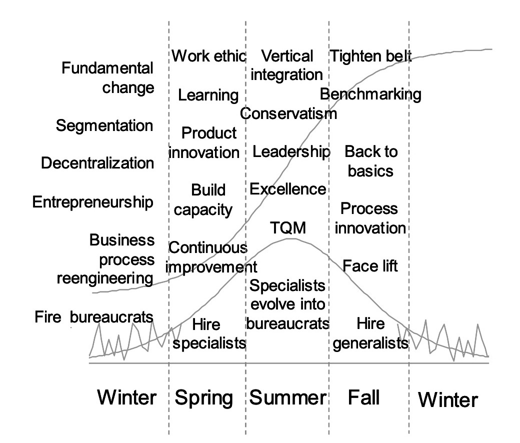
Figure 1: Typical attributes of a growth cycle’s ‘seasons’. Adopted from Modis (1998) with the permission from the author.
Focusing on what to do is appropriate in spring, whereas in fall the emphasis shifts to the how. For example, the evolution of classical music followed a large-timeframe S curve beginning in the fifteenth century and reaching a ceiling in the twentieth century; see Figure 2 (T. Modis, 2013b). In Bach’s time composers were concerned with what to say. The value of their music is in its architecture and as a consequence it can be interpreted by any instrument, even by simple whistling. But two hundred years later composers such as Debussy wrote music that depends crucially on the interpretation, the how. Classical music was still “young” in Bach’s time but was getting “old” by Debussy’s time. No wonder Chopin is more popular than Bartók. Chopin composed during the “summer” of music’s S curve when public preoccupation with music grew fastest. Around that time composers were rewarded more handsomely than today. The innovations they made in music – excursions above the curve – were assimilated by the public within a short period of time because the curve rose steeply and would rapidly catch up with each excursion/innovation. But today the curve has flattened and composers are given limited space. If they make an innovation and find themselves above the curve, there won’t be any time in the future when the public will appreciate their work; see Figure 3 (Modis, 2007). On the other hand, if they don’t innovate, they will not be saying anything new. In either case today’s composers will not be credited with an achievement.
S curves constructed only qualitatively can be accurate, informative, and insightful. Practical challenges of applying S curves are discussed in §3.8.12.
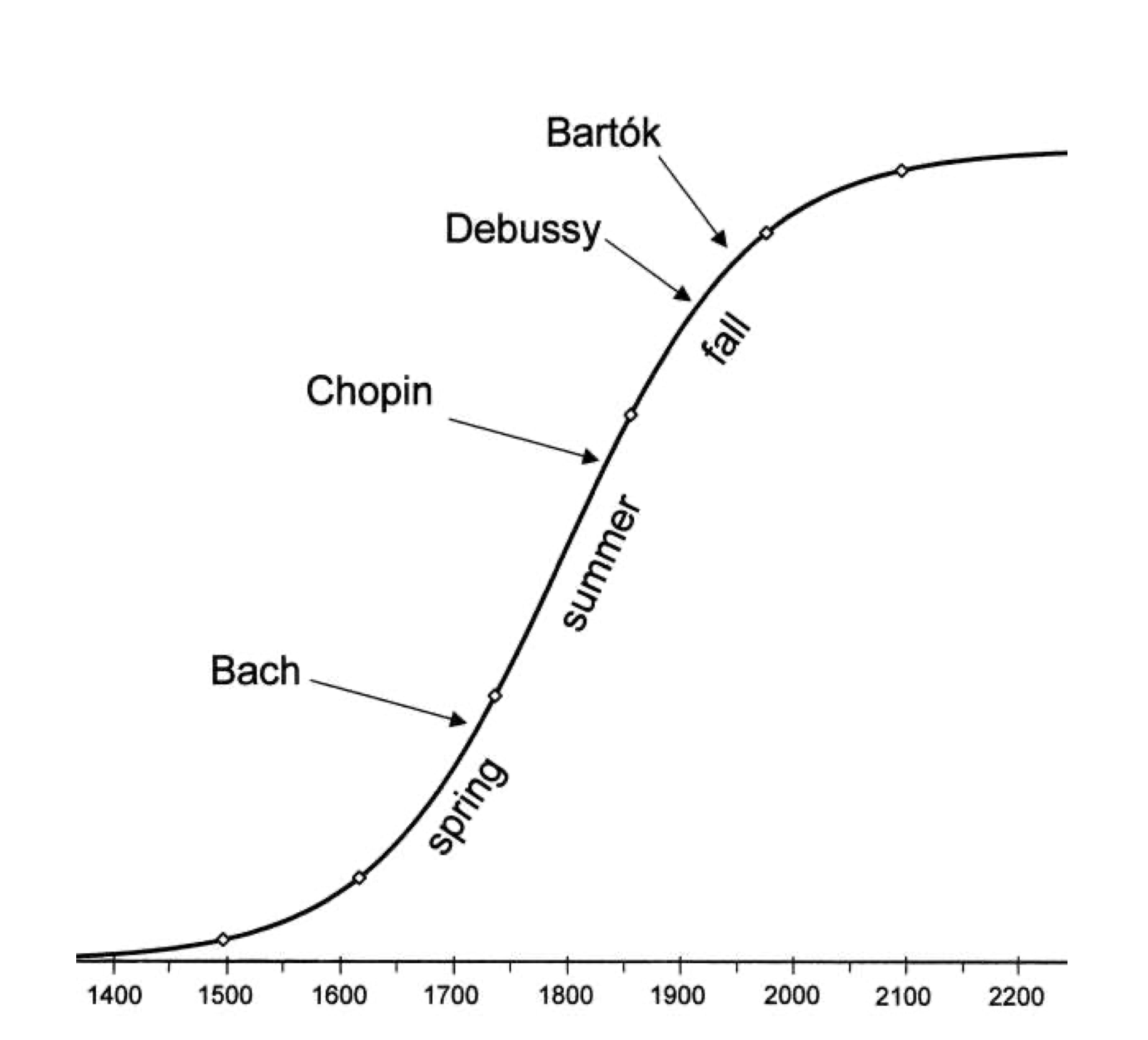
Figure 2: The evolution of classical music. The vertical axis could be something like ‘importance’, ‘public appreciation’, or ‘public preoccupation with music’ (always cumulative). Adopted from T. Modis (2013b) with the permission from the author.
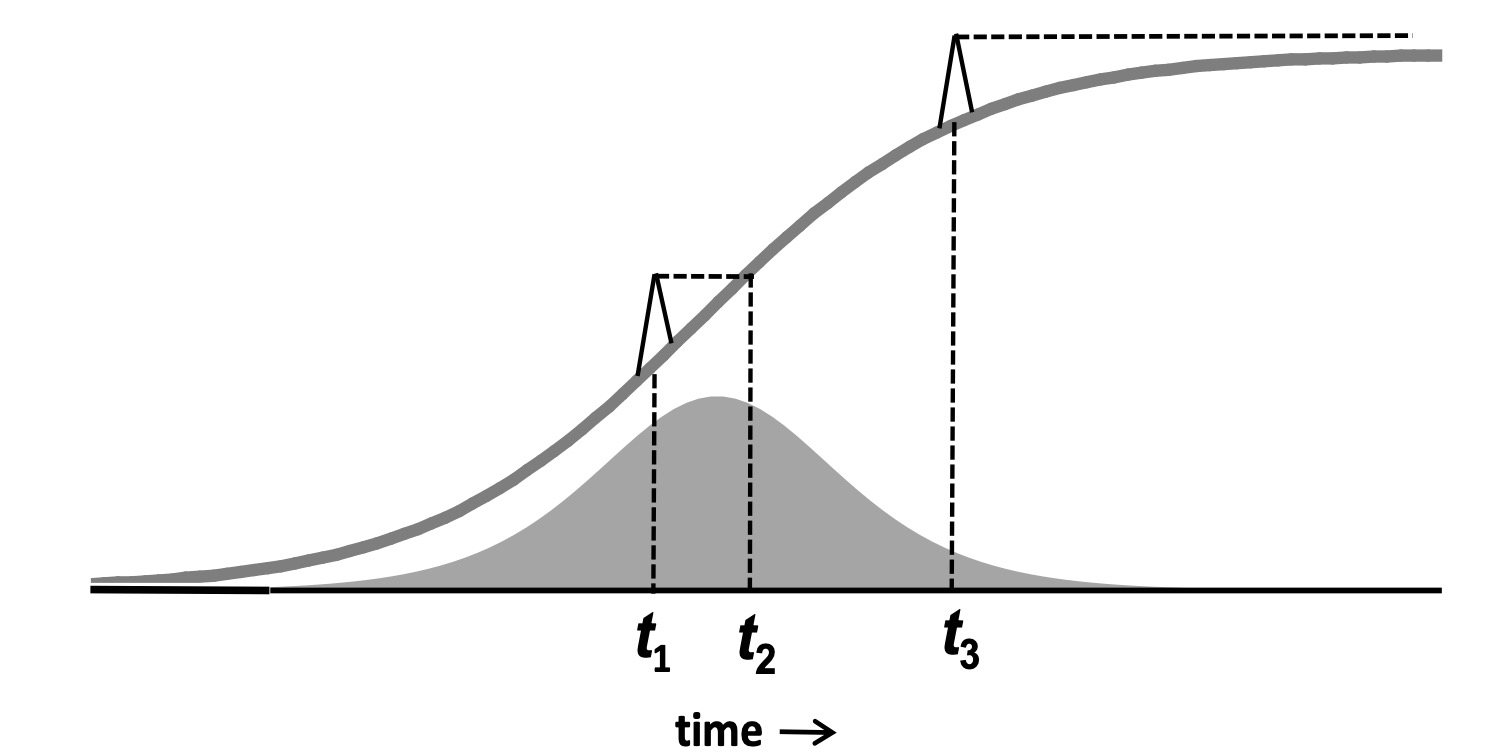
Figure 3: An upward excursion at \(t_1\) reaches the same level as the logistic curve at \(t_2\) and can be considered as a ‘natural’ deviation. The same-size excursion at time \(t_3\) has no corresponding point on the curve. The grey life cycle delimits the position and size of all ‘natural’ deviations. Adapted from Modis (2007) with permission from the author.
There is one more aspect of S curves, recently pointed out, which links them to entropy (amount of disorder) and complexity (Modis, 2022). Entropy’s trajectory grew rapidly during early Universe. As the Universe expansion accelerated, entropy’s growth accelerated. Its trajectory followed a rapidly rising exponential-like growth pattern. At the other end toward the heat death describing the end of the Universe, entropy will grow slowly to asymptotically reach the ceiling of its final maximum (Patel & Lineweaver, 2019). It will most likely happen along another exponential-like pattern. It follows that the overall trajectory of entropy will trace some kind of an S curve with an inflection point somewhere around the middle.
At the same time the complexity of the Universe — if we think of it simply as how difficult it is to describe the Universe — traces out a bell-shaped curve. The very early Universe near the Big Bang was a low-entropy and easy to describe state (low complexity). But the high-entropy state of the end will also be easy to describe because everything will be uniformly distributed everywhere. Complexity was low at the beginning of the Universe and will be low again at the end. It becomes maximal — most difficult to describe — around the middle, the inflection point of entropy’s trajectory, when entropy’s rate of change is maximal; a bell-shaped curve. Complexity’s bell-shaped curve is similar to the time derivative of a logistic function. The implication is that complexity \(C\) is the time derivative of entropy \(S\) (Modis, 2022): \[C = \frac{dS}{dt},\] and \[S = \int C\cdot dt.\]
This relationship is confirmed in a rigorous way with the often-used information-related definitions:
Entropy: the information content.
Complexity: the capacity to incorporate information at a given time.
We see that entropy results from the accumulation (integral) of complexity, or alternatively, that complexity is the time derivative of entropy.
2.3.20 Synchronic and diachronic competition29
Synchronic and diachronic competition models account for critical life cycle perturbations due to interactions, not captured by univariate innovation diffusion models (see §2.3.18) or other time series models, such as ARIMA and VAR. This is important especially in medium and long-term prediction.
Competition in a natural or socio-economic system generally refers to the presence of antagonists that contend for the same resource. This typically occurs in nature, where multiple species struggle with each other to survive, or in socio-economic contexts where products, technologies and ideas concur to be finally accepted within a market and compete for the same market potential. These competition dynamics are reflected in separate time series – one for each concurrent – characterised by a locally oscillatory behaviour with nonlinear trends, unexpected deviations and saturating effects.
The analytic representation of competition has followed different approaches. A first approach has been based on complex systems analysis (Boccara, 2004), which refers to a class of agents (see also §2.7.3) that interact, through local transition rules, and produce competition as an emergent behaviour. This approach may be frequently reduced to a system of differential equations, with suitable mean field approximations. A second approach, systems analysis, has been based on systems of ordinary differential equations (ODE).
In this domain, competition may be a synchronic process, if competitors are present in the environment at the same time; for example, two products may enter the market in the same period. Instead, it is diachronic if competitors come at a later stage; for example, one product enters a market in a given period and just subsequently other similar products enter the same market and start to compete. Pioneering contributions of this competition modelling are due to Lotka (1920) and V. Volterra (1926), who independently obtained a class of synchronic predator-prey models; see also §2.3.19. A generalised version of the Lotka-Volterra (LV) model has been provided by Abramson & Zanette (1998).
Morris & Pratt (2003) proposed an extended LV model for a duopolistic situation, by making explicit the role of carrying capacities or market potentials, and the inhibiting strength of the competitors in accessing the residual resource. LV models typically do not have closed form solutions. In such cases, a staked form of equations allows a first-stage inference based on nonlinear least squares (NLS), with no strong assumptions on the stochastic distributions of error component. Short-term refining may be grounded on a Seasonal Autoregressive Moving Average with exogenous input (SARMAX) representation. Outstanding forecasts may be obtained including the estimated first-stage solution as ‘exogenous’ input (see §2.2.3 and §2.2.5).
A different synchronic model, termed Givon-Bass (GB) model, extending the univariate innovation diffusion models described in §2.3.18 (Bass, 1969; Givon, Mahajan, & Müller, 1995), has been presented in Bonaldo (1991), introducing parametric components of global interaction. In this model, the residual market (or carrying capacity) is completely accessible to all competitors, and the rate equations introduce distributed seeding effects. The GB model has a closed form solution that was independently published by Krishnan, Bass, & Kummar (2000). The more general model by Savin & Terwiesch (2005) and related advances by R. Guseo & Mortarino (2010) were extended to the diachronic case in Guseo & Mortarino (2012), defining a competition and regime change diachronic (CRCD) model with a closed form solution. A relevant improvement of CRCD has been proposed in Guseo & Mortarino (2014), by introducing within-brand and cross-brand word-of-mouth effects, not present in standard LV models. The unrestricted unbalanced diachronic competition (unrestricted UCRCD) model, is defined with these new factors. The model assumes, among other specifications, a constant market potential. In Guseo & Mortarino (2015) this assumption is relaxed, by introducing a dynamic market potential (Guseo & Guidolin, 2009, 2011). Some applications are summarised in §3.8.8.
2.3.21 Estimation and representation of uncertainty30
Forecasting uncertainty consists in estimating the possible range of forecast errors (or true values) in the future and the most widely adopted representation is a forecast interval (Patel, 1989). The forecast interval indicates a range of values and the respective probability, which is likely to contain the true value (which is yet to be observed) of the response variable. Since for a specific lead-time the forecast interval only encompasses information from a marginal distribution, it can also be named marginal forecast interval (MFI). A MFI can be obtained from: parametric distribution, such as a Gaussian distribution with conditional mean and variance estimated with a Generalised ARCH model (Baillie & Bollerslev, 1992); non-parametric distribution, e.g., obtained with conditional kernel density estimation (Rob J. Hyndman et al., 1996); directly estimated with statistical learning methods, such as quantile regression (Taylor & Bunn, 1999) or bootstrapping (Masarotto, 1990), or with machine learning algorithms like quantile random forests (Meinshausen, 2006). For a combination of density forecasts from different models, see §2.6.2.
For multi-zstep ahead forecasting problems (see also §2.7.7), in particular when information about forecast uncertainty is integrated in multi-period stochastic optimisation (Dantzig & Infanger, 1993), information about the temporal dependency structure of forecast errors (or uncertainty) is a fundamental requirement. In this case, the concept of simultaneous forecast intervals (SFI) can be found in the statistical literature (Chew, 1968). SFI differ from MFI since take into account the temporal interdependency of forecast errors and are constructed to have the observed temporal trajectory of the response variable fully contained inside the forecast intervals during all lead-times of the time horizon. The number of works that cover SFI is lower when compared to the MFI, but some examples are: methods based on Bonferroni- and product-type inequalities applied time series forecasting models likes ARIMA and Holt-Winters (Ravishanker, Wu, & Glaz, 1991); combination of bootstrap replications and an heuristic optimisation procedure to find an envelope of the temporal trajectories closest to the deterministic forecast (Staszewska‐Bystrova, 2011 see also §2.7.5); sampling forecast errors at different horizons and estimate the SFI with the empirical Mahalanobis distance (Jordá, Knüppelc, & Marcellino, 2013).
Advances in Operations Research for decision-making problems under uncertainty imposed new requirements in forecast uncertainty estimation and representation. On one hand, stochastic optimisation requires a scenario representation for forecast uncertainty (Powell, 2019). This motivated research in methods that generate uncertainty forecasts represented by random vectors (term used in statistics) or path forecasts (term used in econometrics), such as parametric copula combined with MFI (Pinson, Madsen, Nielsen, Papaefthymiou, & Klöckl, 2009), parametric dynamic stochastic model (J. S.-H. Li & Chan, 2011) or epi-spline basis functions (Rios, Wets, & Woodruff, 2015). On the other hand, robust optimisation does not make specific assumptions on probability distributions and the uncertain parameters are assumed to belong to a deterministic uncertainty set. Hence, some authors proposed new methods to shape forecast uncertainty as polyhedral or ellipsoidal regions to enable a direct integration of forecasts in this type of optimisation problem (Bertsimas & Pachamanova, 2008; Golestaneh, Pinson, & Gooi, 2019).
Finally, communication of forecast uncertainty (e.g., MFI, SFI, random vectors) to decision-makers requires further attention since it remains as a major bottleneck for a wide adoption by industry, particularly in uses cases with multivariate time series (Akram, Binning, & Maih, 2015) and adverse weather events (Ramos, Mathevet, Thielen, & Pappenberger, 2010). Please also see §3.7.5.
2.3.22 Forecasting under fat tails31
A non-negative continuous random variable \(X\) is fat-tailed, if its survival function \(S(x)=P(X\geq x)\) is regularly varying, that is to say if \(S(x)=L(x) x^{-\alpha}\), where \(L(x)\) is a slowly varying function, for which \(\lim_{x \to \infty}\frac{L(tx)}{L(x)}=1\) for \(t>0\) (Embrechts, Klüppelberg, & Mikosch, 2013). The parameter \(\alpha\) is known as the tail parameter, and it governs the thickness of the tail – the smaller \(\alpha\) the fatter the tail – and the existence of moments, so that \(E[X^p]<\infty\) if and only if \(\alpha>p\). Often \(\alpha\) is re-parametrised as \(\xi=1/\alpha\).
Fat tails are omnipresent in nature, from earthquakes to floods, and they are particularly common in human-related phenomena like financial markets, insurance, pandemics, and wars (see, for example, Mandelbrot, 1983; Nassim Nicholas Taleb, 2020 and references therein).
Forecasting fat-tailed random variables is therefore pivotal in many fields of life and science. However, while a basic coverage of the topic is available in most time series and risk management manuals (e.g., Shumway & Stoffer, 2017; McNeil, Frey, & Embrechts, 2015), the profound implications of fat tails are rarely taken into consideration, and this can generate substantial errors in forecasts.
As observed in N N Taleb et al. (2020), any statistical forecasting activity about the mean – or another quantity – of a phenomenon needs the law of large numbers (LLN), which guarantees the convergence of the sample mean at a given known rate, when the number of observations \(n\) grows.
Fat-tailed phenomena with tail parameter \(\alpha \leq 1\) are trivially not predictable. Since their theoretical mean is not defined, the LLN does not work, for there is nothing the sample mean can converge to. This also applies to apparently infinite-mean phenomena, like pandemics and wars, i.e., extremely tricky objects of study, as discussed in P. Cirillo & Taleb (2016a). In similar situations, one can rely on extreme value theory to understand tail risk properties, but should refrain from standard forecasting.
For random variables with \(1<\alpha \leq 2\), the LLN can be extremely slow, and an often unavailable number of observations is needed to produce reliable forecasts. Even for a well-behaved and non-erratic phenomenon, we all agree that a claim about the fitness or non-fitness of a forecasting approach, just on the basis of one single observation (\(n=1\)), would be considered unscientific. The fact is that with fat-tailed variables that “\(n=1\)” problem can be made with \(n=10^6\) observations (Embrechts et al., 2013; Nassim Nicholas Taleb, 2020). In the case of events like operational losses, even a larger \(n\to \infty\) can still be just anecdotal (P. Cirillo & Taleb, 2016a).
According to Nassim Nicholas Taleb (2020), owing to preasymptotics, a conservative heuristic is to manage variables with \(\alpha\leq 2.5\) as practically unpredictable (for example, see §3.6.2 and §3.6.6). Their sample average is indeed too unstable and needs too many observations for forecasts to be reliable in a reasonable period of time. For \(\alpha >2.5\), conversely, forecasting can take place, and the higher \(\alpha\) the better. In any case, more research is strongly needed and desirable (see also §4).
Observe that even discussing the optimality of any alarm system (see, for example, Turkman & Turkman, 1990; Svensson, Holst, Lindquist, & Lindgren, 1996) based on average forecasts would prove meaningless under extremely fat tails (\(\alpha \leq 2\)), when the LLN works very slowly or does not work. In fact, even when the expected value is well-defined (i.e., \(1<\alpha<2\)), the non-existence of the variance would affect all the relevant quantities for the verification of optimality (De Mare, 1980), like for instance the chance of undetected events. For all these quantities, the simple sample estimates commonly used would indeed be misleading.
2.4 Bayesian forecasting
2.4.1 Foundations of Bayesian forecasting32
The Bayesian approach to forecasting produces, by default, a probabilistic forecast (see also §2.6.2 and §2.12.4) describing the uncertainty about future values of the phenomenon of interest, conditional on all known quantities; and with uncertainty regarding all unknown quantities having been integrated out. In order to produce such forecasts, the Bayesian approach requires (i) a predictive model for the future value of the relevant phenomenon, conditional on the observed data and all model unknowns; (ii) a model for the observed data; and (iii) a distribution describing the (subjective or objective) prior beliefs regarding the model unknowns. Using these quantities, the standard calculus of probability distributions, and Bayes’ theorem, then yield the Bayesian predictive (equivalently, forecast) density function (where density is used without loss of generality).
Stated more formally, given observed data up to time \(n\), \(\mathbf{y}=(y_{1},\dots,y_{n})'\), and denoting the model unknowns by \(\theta\), Bayesian forecasting describes the behaviour of the future random variable \(Y_{n+1}\) via the predictive density: \[\begin{equation} p(y_{n+1}|\mathbf{y})=\int p(y_{n+1}|\theta,\mathbf{y})p(\theta|\mathbf{y})d\theta\mathbf{,} \tag{2} \end{equation}\]
where \(y_{n+1}\) denotes a value in the support of \(Y_{n+1}\) and \(p(y_{n+1}|\theta,\mathbf{y})\) is the predictive model for \(Y_{n+1}\) conditional on \(\mathbf{y}\) and the model unknowns \(\theta\). Critically, and in contrast with frequentist approaches to forecasting, parameter uncertainty has been factored into \(p(y_{n+1}|\mathbf{y})\) via the process of integration with respect to the posterior probability density function (pdf) for \(\theta\), \(p(\theta|\mathbf{y})\). The posterior pdf is given, by Bayes’ theorem, as \(p(\theta|\mathbf{y})\propto p(\mathbf{y}|\theta)\times p(\theta),\) where \(p(\mathbf{y}|\theta)\) defines the assumed model for \(\mathbf{y}\) (equivalently, the likelihood function), and the prior pdf \(p(\theta)\) captures prior beliefs about \(\theta.\) Moreover, uncertainty about the assumed predictive model itself can be easily accommodated using Bayesian model averaging, which involves taking a weighted average of model-specific predictives, with posterior model probabilities (also obtained via by Bayes’ theorem) serving as the weights. See Koop (2003), O’Hagan & Forster (2004) and Greenberg (2008) for textbook illustrations of all of these steps.
No matter what the data type, the form of predictive model, or the dimension of the unknowns, the basic manner in which all Bayesian forecast problems are framed is the same. What differs however, from problem to problem, is the way in which the forecasting problem is solved. To understand why, it is sufficient to recognise that in order to obtain the predictive density \(p(y_{T+1}|\mathbf{y})\) we must be able to (somehow) perform the integration that defines this quantity. In almost any practical setting, this integration is infeasible analytically and we must rely on computational methods to access the predictive density. Therefore, the evolution of the practice of Bayesian forecasting has gone hand in hand with developments in Bayesian computation (Martin, Frazier, & Robert, 2020). Through the lens of computation, in §2.4.2 we briefly describe the methods of implementing Bayesian forecasting.
2.4.2 Implementation of Bayesian forecasting33
If the posterior is accessible via methods of exact simulation – e.g., Monte Carlo simulation, importance sampling, Markov chain Monte Carlo (MCMC) sampling, pseudo-marginal MCMC (Andrieu, Doucet, & Holenstein, 2011; Andrieu & Roberts, 2009) – an estimate of the predictive density \(p(y_{n+1}|\mathbf{y})\) in Equation (2) can be produced using draws of the unknown \(\theta\) from the posterior pdf, \(p(\theta|\mathbf{y})\). In most cases, this simulation-based estimate of \(p(y_{n+1}|\mathbf{y})\) can be rendered arbitrarily accurate by choosing a very large number of posterior draws; hence the use of the term ‘exact predictive’ to reference this estimate. See Geweke & Whiteman (2006) for an early review of Bayesian forecasting implemented using exact simulation, §2.3.15, §2.4.3, §2.5.3, §3.3.2, and §3.3.10 for further discussions and a range of relevant applications, and Chapters 3, 7, and 9 in Geweke et al. (2011) for applications in (general) state space, macroeconometric and finance settings respectively. In addition, a 2008 special issue of International Journal of Forecasting on Bayesian Forecasting in Economics provides coverage of forecasting applications (and methods of computation) that exploit exact simulation methods, as do selected chapters in O’Hagan & West (2010) and Brooks, Gelman, Jones, & Meng (2011).
In cases where the posterior is not readily accessible, due to either the intractability of the likelihood function or the high dimension of the model unknowns, or both, methods of approximation are required. Frazier et al. (2019), for instance, produce an ‘approximate predictive’ by replacing the exact posterior in Equation (2), \(p(\theta|\mathbf{y})\), with an ‘approximate posterior’ constructed using approximate Bayesian computation (ABC – Sisson, Fan, & Beaumont, 2019). In large samples, this approximate predictive is shown to be equivalent to the exact predictive. The approximate and exact predictives are also shown to be numerically indistinguishable in finite samples, in the cases investigated; see also Canale & Ruggiero (2016), and Kon Kam King, Canale, & Ruggiero (2019). Related work produces an approximate predictive by exploiting variational Bayes (Blei, Kucukelbir, & McAuliffe, 2017) approximations of the posterior (Chan & Yu, 2020; Koop & Korobilis, 2018; Rubén Loaiza-Maya et al., 2020; Quiroz, Nott, & Kohn, 2018; Tran, Nott, & Kohn, 2017). The flavour of this work is broadly similar to that of Frazier et al. (2019); that is, computing the predictive \(p(y_{n+1}|\mathbf{y})\) via an approximation to the posterior does not significantly reduce predictive accuracy.
The Bayesian paradigm thus provides a very natural and coherent approach to prediction that can be implemented successfully via one of any number of computational methods. Inherent to the approach, however, is the assumption that the model we are using to make predictions is an accurate description of the data generating process (DGP) that has generated the observed data; or if we are averaging across models using Bayesian model averaging, we must assume that this average contains the DGP for the observed data. In response to this limitation, allied with the desire to drive prediction by user-specified measures of predictive loss, new approaches to Bayesian prediction have recently been proposed, and we briefly discuss two such classes of methods.
First are methods for combining predictives in which the weights are not equated to the posterior model probabilities (as in standard Bayesian model averaging) but, rather, are updated via problem-specific predictive criteria, or via predictive calibration (Dawid, 1982, 1985; Gneiting et al., 2007); see Billio, Casarin, Ravazzolo, & van Dijk (2013), Casarin, Leisen, Molina, & Horst (2015), Pettenuzzo & Ravazzolo (2016), Bassetti, Casarin, & Ravazzolo (2018), Basturk, Borowska, Grassi, Hoogerheide, & Dijk (2019), McAlinn & West (2019), and McAlinn, Aastveit, Nakajima, & West (2020), for a selection of approaches, and §2.6.2 for related discussion. Importantly, these methods do not assume the true model is spanned by the constituent model set. Second are methods in which the standard Bayesian posterior, which is itself based on a potentially misspecified model, is replaced by a generalised version that is designed for the specific predictive task at hand (e.g., accurate prediction of extreme values); with the overall goal then being to produce predictions that are accurate according to the particular measure of interest. See Syring & Martin (2020), Ruben Loaiza-Maya et al. (2020), and Frazier, Loaiza-Maya, Martin, & Koo (2021) for specific examples of this methodology, as well as proofs of its theoretical validity.
2.4.3 Bayesian forecasting with copulas34
Copulas provide intrinsic multivariate distribution structure that allows for modelling multivariate dependence with marginal distributions as the input, making it possible to forecast dependent time series and time series dependence. This review focuses on the Bayesian approach for copula forecasting. For rigorous topics on copula introduction (Joe, 1997; Nelsen, 2006; Trivedi & Zimmer, 2007), copula modelling techniques (Durante & Sempi, 2015), vine copulas (Joe, 2014), review on frequentist approaches for copula-based forecasting (Patton, 2013), see the aforementioned references and the references therein.
The advantages of the Bayesian copula approach compared to the frequentist treatments are (i) the Bayesian approach allows for jointly modelling the marginal models and the copula parameters, which improves the forecasting efficiency (Joe, 2005; Li & Kang, 2018), (ii) probabilistic forecasting is naturally implied with the Bayesian predictive density, and (iii) experts information can be seamlessly integrated into forecasting via the priors’ setting.
Forecasting with copulas involves selecting between a different class of copulas. Common approaches include Bayesian hypothesis testing (see §2.4.1) where copula parameters are treated as nuisance variables (Huard, Évin, & Favre, 2006), or parsimonious modelling of covariance structures using Bayesian selection and model averaging (Min & Czado, 2011; Pitt, Chan, & Kohn, 2006; Smith, 2010).
One particular interest in copulas is to forecast the dynamic dependencies between multivariate time series. Time-varying copula construction is possible via (i) an autoregressive or GARCH form (see §2.3.11) of dependence parameters (Lucas, Schwaab, & Zhang, 2014; A. J. Patton, 2006), (ii) factor copula construction (Oh & Patton, 2018; Tan, Panagiotelis, & Athanasopoulos, 2019) that simplifies the computation, (iii) the stochastic copula autoregressive model (Almeida & Czado, 2012) that dependence is modelled by a real-valued latent variable, and (iv) covariate-dependent copulas approach by parameterising the dependence as a function of possible time-dependent covariates (Li & Kang, 2018) that also improves the forecasting interpretability. ARMA-like and GARCH-like dependences in the tail can be considered as special cases of (Li & Kang, 2018).
In multivariate time series forecasting (see also §2.3.9), unequal length of data is a common issue. One possible approach is to partition the copula parameters into elements relating only to the marginal distributions and elements only relating to the copula (Patton, 2006). For mixed frequency data, it is possible to decompose the copula dependence structure into linear and nonlinear components. Then the high and low frequency data is used to model the linear and nonlinear dependencies, respectively (Oh & Patton, 2016). Bayesian data augmentation is also used to forecast multivariate time series with mixed discrete and continuous margins (Smith & Khaled, 2012). For other treatments for discrete and continuous time series (see, for example, Panagiotelis, Czado, & Joe, 2012; Panagiotelis, Czado, Joe, & Stöber, 2017).
Bayesian approach for lower dimensional copula forecasting (\(d < 10\)) is straightforward with traditional Gaussian copulas, Student’s-\(t\) copulas, Archimedean copulas, or pair copula combinations. In higher dimensional settings, special considerations are required to save the computational burden, such as low rank approximation of covariates matrix (Salinas et al., 2019a) or factor copula models with stochastic loadings (Creal & Tsay, 2015).
In the Bayesian setup, forecasting model performance is typically evaluated based on a \(K\)-fold out-of-sample log predictive score (LPS: Geweke & Amisano, 2010), and out-of-sample Value-at-Risk (VaR) or Expected Shortfall (ES) are particularly used in financial applications. The LPS is an overall forecasting evaluation tool based on predictive densities, serving out-of-sample probabilistic forecasting. LPS is ideal for decision makers (Geweke, 2001; Geweke & Amisano, 2010). The VaR gives the percentile of the conditional distribution, and the corresponding ES is the expected value of response variable conditional on it lying below its VaR.
2.5 Variable and model selection
2.5.1 Leading indicators and Granger causality35
Leading (economic) indicators are variables that try to capture changes in the development of economic activity before those changes materialise. Typically, market participants, policy makers, the general public, etc. are interested in which direction the economy of a country is developing ahead of the publication date of the respective quarterly GDP figures (see also §3.3.2), for which these leading indicators play a crucial role. This is of particular relevance for short-term forecasting and nowcasting of such a (low-frequency) variable characterised by a publication lag.
For some leading indicators, single variables are combined into a composite index such as The Conference Board Leading Economic Index published by The Conference Board for the United States. It consists of averages of ten variables, including average weekly hours in manufacturing, manufacturers’ new orders, private housing building permits, and average consumer expectations (The Conference Board, 2020). Other leading indicators consist of one variable only and are purely survey-based, such as the monthly ifo Business Climate Index published by the ifo Institute for Germany, which covers the appraisal of current and future expected business of executives of approximately 9,000 German firms across industries (ifo Institute, 2020).
If a specific leading indicator is able to capture certain economic changes before they happen, such a leading indicator \(x_t\) is said to Granger-cause (or predictively cause) a forecast variable \(y_t\) (Granger, 1969), implying that a “cause” cannot happen after an effect. In (theoretical) econometric terms and following the notation of Lütkepohl (2005), \(y_t\) is Granger-caused by \(x_t\) if for at least one forecast horizon \(h=1, 2, \dots\) the following inequality holds: \[\sum_{y}(h \mid \Omega_i) < \sum_{y}(h \mid \Omega_i \setminus \{x_t \mid t \leq i \}).\]
In other words, the mean square error of the optimal \(h\)-step-ahead predictor of the forecast variable, which includes the information contained in the leading indicator in the set of all relevant information to the forecaster available at the forecast origin \(\sum_{y}(h \mid \Omega_i)\), must be smaller than the mean square error of that \(h\)-step-ahead predictor of the forecast variable without the information contained in said leading indicator \(\sum_{y}(h \mid \Omega_i \setminus \{x_t \mid t \leq i \})\) (Lütkepohl, 2005).
Nonetheless, the concept of Granger causality also has its limitations. The notion that a “cause” cannot happen after an effect is only a necessary, yet not a sufficient condition for causality, hence the reason why “cause” has been written with quotation marks in this section. If one ignored this fact and equated causality with Granger causality, they would commit an informal logical fallacy called Post hoc ergo propter hoc (i.e., after this, therefore because of this; Walton, Reed, & Macagno, 2008). A bold example of this fallacy would be, “Because the birds migrate, winter is coming”. This is a fallacy, as winter would come at about the same time every year, no matter if there were migrating birds or not. Moreover, hardly any economic activity is monocausal.
There are also different types of formal statistical Granger causality tests available for different data structures that are implemented in typical statistics/econometrics software packages. For the simple case of two variables (Granger, 1969), say the forecast variable and the leading indicator, the null hypothesis of a bivariate Granger causality test is that the leading indicator does not Granger-cause the forecast variable. Under this null hypothesis, the \(F\)-test statistic on the joint impact of the coefficients of the past realisations of the leading indicator employed as explanatory variables in a multiple linear regression with the forecast variable as dependent variable and its past realisations as additional explanatory variables will not be statistically significantly different from zero. The maximum lag for past realisations would be optimally determined, for instance, by some information criterion (e.g., AIC, BIC; see also §2.5.4). Practical applications of Granger causality and leading indicators in tourism demand forecasting can be found, for instance, in §3.8.1.
2.5.2 Model complexity36
A simple model must be easily understood by decision-makers. On the contrary, relationships in a complex model are opaque for its users (see also §3.7.4). In this context, complexity is not measured solely by the number of parameters, but also by the functional form of the relationships among variables.
Complex models are commonly believed to deliver better forecasts, as they well describe sophisticated economic structures and offer good fit the data. Consequently, they are favoured by researchers, decision-makers and academic journals. However, empirical studies provide little evidence about their forecasting superiority over simple models. This can be explained using the bias-variance trade-off framework, in which the mean squared error can be decomposed into \[MSE = noise + variance + bias^2.\] Noise is driven by the random term in the model. It cannot be avoided, even if we know the true DGP. Variance is caused by the need to estimate the model parameters, hence its value increases with model complexity and declines with the sample size. Bias is predominantly related to model mis-specification, which is most likely to occur for simple methods. The implications of the above framework are twofold: (i) the relationship between model complexity and MSE is U-shaped and (ii) the optimal model complexity increases with the sample size.
The illustration of the bias-variance trade-off for a simple autoregressive model (see §2.3.4) is provided by Ca’ Zorzi, Muck, & Rubaszek (2016). They present analytical proof that for any persistent DGP of the form \(y_t=c+\phi y_{t-1}+\epsilon_t\) characterised by half-life of over two years, the accuracy of forecasts from the random walk or the AR(1) model with parameter \(\phi\) fixed at an arbitrary value consistent with half-life of five years tend to be higher than that from the estimated AR(1) model. This result explains why in numerous studies the random walk is a tough benchmark as well as why a simple, calibrated AR(1) model can be successful in forecasting inflation (Faust & Wright, 2013), exchange rates (Ca’ Zorzi, Kolasa, & Rubaszek, 2017) or oil prices (Rubaszek, 2020) compared to a number of complex competitors.
Wide support to the view that model simplicity improves forecasting performance is presented by Green & Armstrong (2015), in an introductory article to the special issue of Journal of Business Research “Simple versus complex forecasting”, as well as the results of M1 and M2 competitions (Makridakis et al., 1982, 1993). Stock & Watson (1998) also show that for most US monthly series complex non-linear autoregressive models deliver less accurate forecasts than their linear counterparts. On the contrary, the results of M4 competition tend to favour more complex models (Spyros Makridakis et al., 2020b and §2.12.7).
Why are then complex models preferred to simple ones, if the latter deliver more accurate forecasts? Brighton & Gigerenzer (2015) claim that there is a tendency to overemphasize the bias component and downplay the role of variance. This behaviour is leading to an implicit preference towards more complex forecasting methods, which is called by the authors as “bias bias”. To avoid it, one can follow the golden rules of forecasting, which says: be conservative in the choice of over-ambitious models and be wary of the difficulty to forecast with complex methods (Armstrong, Green, & Graefe, 2015). The alternative is to use methods, which explicitly account for the bias-variance trade-off, e.g. machine learning (see §2.7.10).
2.5.3 Variable selection37
References to ‘big data’ have become somewhat ubiquitous both in the media and in academic literature in recent years (see §2.7.1 but also §2.2.5). Whilst in some disciplines (for example Finance) it has become possible to observe time series data at ever higher frequency, it is in the cross section that the amount of data available to analysts has seen exponential growth.
Ordinary Least Squares (OLS) is the standard tool for data analysis and prediction, but is well known to perform poorly when there many potential explanatory variables; Bishop (2006) sets out clearly why this is so. In situations where there is no obvious underlying model to suggest which of a potentially large set of candidate variables to focus on, the researcher needs to add new tools to the tool kit.
There are two principal sets of approaches to this problem. The first seeks to reduce the model dimensions by summarising the predictors in to a much smaller number of aggregated indices or factors. The second is to employ a regularisation strategy to reduce the effective dimension of the problem by shrinking the size of the regression coefficients. Some strategies reduce a subset of these coefficients to zero, removing some variables from the model entirely and these can hence be described as variable selection procedures.
Such procedures may be applicable either when a problem is believed to be truly sparse, with only a small number of variables having an effect, or alternatively when a sparse model can provide effective forecasts, even though the underling system is in fact more complex (see also §2.5.2).
In the frequentist framework, the Least Absolute Shrinkage and Selection Operator (LASSO) procedure of Tibshirani (1996) has proven effective in many applications. The LASSO requires choice of an additional regularisation parameter (usually selected by some statistical criteria or via a cross validation process). Various refinements to the original LASSO procedure have been developed, see in particular Rapach, Strauss, Tu, & Zhou (2019) for a recent forecasting application. An alternative frequentist approach to variable selection and shrinkage is the Complete Subset Regression (CSR) model of Elliott (2015), where separate OLS regressions are run on all possible combinations of potential regressors, with forecasts generated by averaging across the entire set of models. Kotchoni, Leroux, & Stevanovic (2019) combine CSR with LASSO in a comprehensive empirical economic forecasting exercise.
Where the underlying process is not properly sparse (see Giannone & Primiceri, 2017 for a discussion), it is perhaps more natural to work in a Bayesian framework where samples can be drawn from the variable selection part of model reflecting the estimated probability of inclusion of each variable. The appropriate degree of regularisation can also be selected in a similar way. Forecasts are then constructed as weighted averages over several sparse models. This approach has proven to be very effective in practice, for example in fitting Bayesian Vector Auto Regressions to forecast economic time series. Early examples include George & McCulloch (1993) and Mitchell & Beauchamp (1988), which use binary indicators to select variables in to the model. More recent approaches use continuous random variables to achieve a similar effect, making computation more tractable. Examples include the Horeshoe Prior (Carvalho, Polson, & Scott, 2010; Piironen & Vehtari, 2017) and the LN-CASS prior of Thomson, Jabbari, Taylor, Arlt, & Smith (2019). Cross (2020) is a recent example of an economic forecasting exercise using several such models.
2.5.4 Model selection38
Taxonomies of all possible sources of forecast errors from estimated models that do not coincide with their data generating process (DGP) have revealed that two mistakes determine forecast failures (i.e., systematic departures between forecasts and later outcomes), namely mis-measured forecast origins and unanticipated location shifts (Clements & Hendry, 1999; Hendry & Mizon, 2012). The former can be addressed by nowcasting designed to handle breaks (BańBura, Giannone, & Reichlin, 2011; J. L. Castle & Hendry, 2010; J. L. Castle et al., 2018b). It is crucial to capture the latter as failure to do so will distort estimation and forecasts, so must be a focus when selecting models for forecasting facing an unknown number of in-sample contaminating outliers and multiple breaks at unknown times.
Consequently, selection must be jointly over both observations and variables, requiring computer learning methods (J. L. Castle et al., 2020b see also §3.6.2; Hendry & Doornik, 2014). Autometrics, a multiple-path block-search algorithm (see Doornik (2018)), uses impulse (IIS: D. F. Hendry et al. (2008a) and Johansen & Nielsen (2009)) and step (SIS: J. L. Castle et al. (2015b)) indicator saturation for discovering outliers and breaks, as well as selecting over other variables. Although knowing the in-sample DGP need not suffice for successful forecasting after out-of-sample shifts, like financial crises and pandemics, ‘robust variants’ of selected models can then avoid systematic mis-forecasts (see, for example, Martinez et al., 2021; Doornik et al., 2020a and §3.3.4).
Saturation estimation has approximately \(K=k+2n\) candidates for \(k\) regressors, with \(2^K\) possible models, requiring selection with more candidate variables, \(K\), than observations, \(n\) (also see §2.7 and §2.3.9). Selection criteria like AIC (Akaike, 1973), BIC (Schwarz, 1978), and HQ (Hannan & Quinn, 1979) are insufficient in this setting. For saturation estimation, we select at a tight significance level, \(\alpha=1/K\), retaining subject-theory variables and other regressors. When forecasting is the aim, analyses and simulations suggest loose significance for then selecting other regressors, close to the 10% to 16% implied significance level of AIC, regardless of location shifts at or near the forecast origin (J. L. Castle et al., 2018a). At loose levels, Autometrics can find multiple undominated terminal models across paths, and averaging over these, a univariate method and a robust forecasting device can be beneficial, matching commonly found empirical outcomes. The approach applies to systems, whence selection significance of both indicators and variables is judged at the system level. Capturing in-sample location shifts remains essential (J. A. Doornik et al., 2020b).
There are costs and benefits of selection for forecasting (also see §2.5.3 and §2.11.3). Selection at a loose significance level implies excluding fewer relevant variables that contribute to forecast accuracy, but retaining more irrelevant variables that are adventitiously significant, although fewer than by simply averaging over all sub-models (Hoeting, Madigan, Raftery, & Volinsky, 1999). Retaining irrelevant variables that are subject to location shifts worsens forecast performance, but their coefficient estimates are driven towards zero when updating estimates as the forecast origin moves forward. Lacking omniscience about future values of regressors that then need to be forecast, not knowing the DGP need not be costly relative to selecting from a general model that nests it (Castle et al., 2018a). Overall, the costs of model selection for forecasting are small compared to the more fundamental benefit of finding location shifts that would otherwise induce systematic forecast failure.
2.5.5 Cross-validation for time-series data39
When building a predictive model, its purpose is usually not to predict well the already known samples, but to obtain a model that will generalise well to new, unseen data. To assess the out-of-sample performance of a predictive model we use a test set that consists of data not used to estimate the model (for a discussion of different error measures used in this context see §2.12.2). However, as we are now using only parts of the data for model building, and other parts of the data for model evaluation, we are not making the best possible use of our data set, which is a problem especially if the amount of data available is limited. Cross-validation (CV), first introduced by Stone (1974), is a widely used standard technique to overcome this problem (Hastie et al., 2009) by using all available data points for both model building and testing, therewith enabling a more precise estimation of the generalisation error and allowing for better model selection. The main idea of (\(k\)-fold) cross-validation is to partition the data set randomly into \(k\) subsets, and then use each of the \(k\) subsets to evaluate a model that has been estimated on the remaining subsets. An excellent overview of different cross-validation techniques is given by Arlot & Celisse (2010).
Despite its popularity in many fields, the use of CV in time series forecasting is not straightforward. Time series are often non-stationary and have serial dependencies (see also §2.3.4). Also, many forecasting techniques iterate through the time series and therewith have difficulties dealing with missing values (withheld for testing). Finally, using future values to predict data from the past is not in accordance with the normal use case and therewith seems intuitively problematic. Thus, practitioners often resort to out-of-sample evaluation, using a subset from the very end of a series exclusively for evaluation, and therewith falling back to a situation where the data are not used optimally.
To overcome these problems, the so-called time-series cross-validation (Hyndman & Athanasopoulos, 2018) extends the out-of-sample approach from a fixed origin to a rolling origin evaluation (Tashman, 2000). Data is subsequently moved from the out-of-sample block from the end of the series to the training set. Then, the model can be used (with or without parameter re-estimation) with the newly available data. The model re-estimation can be done on sliding windows with fixed window sizes or on expanding windows that always start at the beginning of the series (Bell & Smyl, 2018).
However, these approaches extending the out-of-sample procedure make
again not optimal use of the data and may not be applicable when only
small amounts of data are available. Adapting the original CV procedure,
to overcome problems with serial correlations, blocked CV approaches
have been proposed in the literature, where the folds are chosen in
blocks (Bergmeir & Benı́tez, 2012; Racine, 2000) and/or data
around the points used for testing are omitted
(Burman, Chow, & Nolan, 1994; Racine, 2000). Finally, it has been
shown that with purely autoregressive models, CV can be used without
modifications, i.e., with randomly choosing the folds
(Bergmeir, Hyndman, & Koo, 2018). Here, CV estimates the generalisation error
accurately, as long as the model errors from the in-sample fit are
uncorrelated. This especially holds when models are overfitting.
Underfitting can be easily detected by checking the residuals for serial
correlation, e.g., with a Ljung-Box test (Ljung & Box, 1978). This
procedure is implemented in the forecast package
(R. Hyndman et al., 2020) in R (R Core Team, 2020), in the function CVar.
2.6 Combining forecasts
2.6.1 Forecast combination: a brief review of statistical approaches40
Given \(N\) forecasts of the same event, forecast combination involves estimation of so called combination weights assigned to each forecast, such that the accuracy of the combined forecast generally outperforms the accuracy of the forecasts included. Early statistical approaches adopted a range of strategies to estimate combination weights including (i) minimising in-sample forecast error variance among forecast candidates (Bates & Granger, 1969; Min & Zellner, 1993; Newbold & Granger, 1974), (ii) formulation and estimation via ordinary least squares regression (Granger & Ramanathan, 1984; MacDonald & Marsh, 1994), (iii) use of approaches based on Bayesian probability theory (Bordley, 1982; Bunn, 1975; Clemen & Winkler, 1986; Diebold & Pauly, 1990; Raftery, 1993 and §2.4), (iv) and the use of regime switching and time varying weights recognising that weights can change over time (Diebold & Pauly, 1987; Elliott, Timmermann, & Komunjer, 2005; Lütkepohl, 2011; Tian & Anderson, 2014 and §2.3.12). D. K. Barrow & Kourentzes (2016) contains a very good documentation and empirical evaluation of a range of these early approaches, while De Menezes, Bunn, & Taylor (2000) and Jon Scott Armstrong (2001) contain guidelines on their use.
Recent statistical approaches use a variety of techniques to generate forecasts and/or derive weights. Kolassa (2011) apply so called Akaike weights based on Akaike Information Criterion (Sakamoto, Ishiguro, & Kitagawa, 1986), while bootstrapping has been used to generate and combine forecast from exponential smoothing (Barrow, Kourentzes, Sandberg, & Niklewski, 2020; Bergmeir, Hyndman, & Benı́tez, 2016 but also §2.7.5 and §2.7.6; Cordeiro & Neves, 2009), artificial neural networks (D. K. Barrow & Crone, 2016a, 2016b and §2.7.8), and other forecast methods (Athanasopoulos, Song, & Sun, 2018; Hillebrand & Medeiros, 2010; Inoue & Kilian, 2008). D. K. Barrow & Crone (2016b) developed cross-validation and aggregating (Crogging) using cross-validation to generate and average multiple forecasts, while more recently, combinations of forecasts generated from multiple temporal levels has become popular (Athanasopoulos, Hyndman, Kourentzes, & Petropoulos, 2017; Kourentzes & Athanasopoulos, 2019 and §2.10.2; Kourentzes, Petropoulos, & Trapero, 2014). These newer approaches recognise the importance of forecast generation in terms of uncertainty reduction (Petropoulos et al., 2018a), the creation of diverse forecasts (G. Brown et al., 2005; Lemke & Gabrys, 2010), and the pooling of forecasts (Kourentzes et al., 2019; Lichtendahl Jr & Winkler, 2020).
Now nearly 50 years on from the seminal work of (Bates & Granger, 1969), the evidence that statistical combinations of forecasts improves forecasting accuracy is near unanimous, including evidence from competitions (Makridakis et al., 1982, 2020b and §2.12.7; Makridakis & Hibon, 2000), and empirical studies (Andrawis, Atiya, & El-Shishiny, 2011; Elliott et al., 2005; Jose & Winkler, 2008; Kourentzes et al., 2019). Still, researchers have tried to understand why and when combinations improve forecast accuracy (Atiya, 2020; Palm & Zellner, 1992; Petropoulos et al., 2018a; Timmermann, 2006), and the popularity of the simple average (Chan & Pauwels, 2018; Claeskens, Magnus, Vasnev, & Wang, 2016; J. Smith & Wallis, 2009a). Others have investigated properties of the distribution of the forecast error beyond accuracy considering issues such as normality, variance, and in out-of-sample performance of relevance to decision making (D. K. Barrow & Kourentzes, 2016; Chan, Kingsman, & Wong, 1999; Makridakis & Winkler, 1989).
Looking forward, evidence suggests that the future lies in the combination of statistical and machine learning generated forecasts (Makridakis et al., 2020b), and in the inclusion of human judgment (Gupta, 1994; Petropoulos et al., 2018b but also §2.11.1; Xun Wang & Petropoulos, 2016). Additionally, there is need to investigate such issues as decomposing combination accuracy gains, constructing prediction intervals (Grushka-Cockayne & Jose, 2020; Koenker, 2005), and generating combined probability forecasts (Clements & Harvey, 2011 and §2.6.2; Hall & Mitchell, 2007; Raftery, Madigan, & Hoeting, 1997; Ranjan & Gneiting, 2010). Finally, there is need for the results of combined forecasts to be more interpretable and suitable for decision making (D. K. Barrow & Kourentzes, 2016; Bordignon, Bunn, Lisi, & Nan, 2013; Graefe et al., 2014; Todini, 2018).
2.6.2 Density forecast combinations41
Density forecasts provide an estimate of the future probability distribution of a random variable of interest. Unlike point forecasts (and point forecasts supplemented by prediction intervals) density forecasts provide a complete measure of forecast uncertainty. This is particularly important as it allows decision makers to have full information about the risks of relying on the forecasts of a specific model. Policy makers like the Bank of England, the European Central Bank and Federal Reserve Banks in the US routinely publish density forecasts of different macroeconomic variables such as inflation, unemployment rate, and GDP. In finance, density forecasts find application, in particular, in the areas of financial risk management and forecasting of stock returns (see, for example, Tay & Wallis, 2000; Berkowitz, 2001; Guidolin & Timmermann, 2006; Shackleton, Taylor, & Yu, 2010 inter alia). The reader is referred to §3.3 for a discussion of relevant applications.
Initial work on forecast combination focused on the combination of point forecasts (see §2.6.1). In recent years attention has shifted towards evaluation, comparison and combination of density forecasts with empirical applications that are mostly encountered in the areas of macroeconomics and finance. The improved performance of combined density forecasts stems from the fact that pooling of forecasts allows to mitigate potential misspecifications of the individual densities when the true population density is non-normal. Combining normal densities yields a flexible mixture of normals density which can accommodate heavier tails (and hence skewness and kurtosis), as well as approximate non-linear specifications (Hall & Mitchell, 2007; Jore, Mitchell, & Vahey, 2010).
The predictive density combination schemes vary across studies and range from simple averaging of individual density forecasts to complex approaches that allow for time-variation in the weights of prediction models, also called experts (see Aastveit, Mitchell, Ravazzolo, & Dijk, 2019 for a comprehensive survey of density forecast combination methods). A popular approach is to combine density forecasts using a convex combination of experts’ predictions, so called ‘linear opinion pools’ (see, for example, Hall & Mitchell, 2007; Geweke & Amisano, 2011; Kascha & Ravazzolo, 2010). In order to determine the optimal combination weights this method relies on minimising Kullback-Leibler divergence of the true density from the combined density forecast. These linear approaches have been extended by Gneiting & Ranjan (2013) to allow non-linear transformations of the aggregation scheme and by Kapetanios, Mitchell, Price, & Fawcett (2015), whose ‘generalised pools’ allow the combination weights to depend on the (forecast) value of the variable of interest.
Billio et al. (2013) developed a combination scheme that allows the weights associated with each predictive density to be time-varying, and propose a general state space representation of predictive densities and combination schemes. The constraint that the combination weights must be non-negative and sum to unity implies that linear and Gaussian state-space models cannot be used for inference and instead Sequential Monte Carlo methods (particle filters) are required. More recently, McAlinn & West (2019) developed a formal Bayesian framework for forecast combination (Bayesian predictive synthesis) which generalises existing methods. Specifying a dynamic linear model for the synthesis function, they develop a time-varying (non-convex/nonlinear) synthesis of predictive densities, which forms a dynamic latent (agent) factor model.
For a discussion on methods for evaluating probabilistic forecasts, see §2.12.4 and §2.12.5.
2.6.3 Ensembles and predictive probability post processors42
Improved rational decisions are the final objective of modelling and forecasting. Relatively easy decisions among a number of alternatives with predefined and known outcomes become hard when they are conditioned by future unknown events. This is why one resorts to modelling and forecasting, but this is insufficient. To be successful, one must account for the future conditioning event uncertainty to be incorporated into the decision-making process using appropriate Bayesian approaches (see also §2.4), as described by the decision theory literature (Berger, 1985; Bernardo, 1994; DeGroot, 2004). The reason is that taking a decision purely based on model forecasts is equivalent to assuming the future event (very unlikely, as we know) to equal the forecasted value. Therefore, the estimation of the predictive probability density is the essential prerequisite to estimating the expected value of benefits (or of losses) to be compared and traded-off in the decision-making process (Draper & Krnjajić, 2013). This highly increases the expected advantages together with the likelihood of success and the robustness of the decision (Todini, 2017, 2018).
In the past, the assessment of the prediction uncertainty was limited to the evaluation of the confidence limits meant to describe the quality of the forecast. This was done using continuous predictive densities, as in the case of the linear regression, or more frequently in the form of predictive ensembles. These probabilistic predictions, describing the uncertainty of the model forecasts given (knowing) the observations can be used within the historical period to assess the quality of the models (Todini, 2016). When predicting into the future, observations are no more available and what we look for (known as predictive probability) is the probability of occurrence of the unknown “future observations” given (knowing) the model forecasts. This can be obtained via Bayesian inversion, which is the basis of several uncertainty post-processors used in economy (Diebold, Gunther, & Tay, 1998 and §3.3), hydrology (Krzysztofowicz, 1999; Schwanenberg et al., 2015 and §3.5.4; Todini, 1999, 2008), meteorology (Economou, Stephenson, Rougier, Neal, & Mylne, 2016; Granger & Pesaran, 2000; Katz & Lazo, 2011; Reggiani & Boyko, 2019 see also §3.5.2), etc. Accordingly, one can derive a predictive probability from a single model forecast to estimate the expected value of a decision by integrating over the entire domain of existence all the possible future outcomes and theirs effects, weighted with their appropriate probability of occurrence.
When several forecasts are available to a decision maker, the problem of deciding on which of them one should rely upon becomes significant. It is generally hard to choose among several forecasts because one model could be best under certain circumstances but rather poor under others. Accordingly, to improve the available knowledge on a future unknown event, predictive densities are extended to multiple forecasts to provide decision makers with a single predictive probability, conditional upon several model’s forecasts (G Coccia & Todini, 2011 see also §2.6.1 and §2.6.2; Raftery et al., 1997).
A number of available uncertainty post processors can cope with multi-model approaches, such as Bayesian model averaging (Raftery, 1993; Raftery et al., 1997), model output statistics (Glahn & Lowry, 1972; Wilkd, 2005), ensemble model output statistics (Gneiting, Raftery, Westveld, & Goldman, 2005), and model conditional processor (G Coccia & Todini, 2011; Todini, 2008).
Finally, important questions such as: (i) “what is the probability that an event will happen within the next \(x\) hours?” and (ii) “at which time interval it will most likely occur?” can be answered using a multi-temporal approach (Gabriele Coccia, 2011 see also §2.10.2; Krzysztofowicz, 2014) and results of its applications were presented in Gabriele Coccia (2011), Todini (2017), and Barbetta, Coccia, Moramarco, Brocca, & Todini (2017).
2.6.4 The wisdom of crowds43
Multiple experts’ forecasts are collected in a wide variety of situations: medical diagnostics, weather prediction, forecasting the path of a hurricane, predicting the outcome of an election, macroeconomic forecasting, and more. One of the central findings from the forecasting literature is that there is tremendous power in combining such experts’ forecasts into a single forecast. The simple average, or what Surowiecki refers to as ‘the wisdom of crowds’ (Surowiecki, 2005), has been shown to be a surprisingly robust combined forecast in the case of point forecasting (Armstrong, 2001 and §2.6.1; Clemen, 1989; Clemen & Winkler, 1986). The average forecast is more accurate than choosing a forecast from the crowd at random and is sometimes even more accurate than nearly all individuals (Mannes, Larrick, & Soll, 2012). The average point forecast also often outperforms more complicated point aggregation schemes, such as weighted combinations (J. Smith & Wallis, 2009b; Soule, Grushka-Cockayne, & Merrick, 2020).
Mannes et al. (2012) highlight two crucial factors that influence the quality of the average point forecast: individual expertise and the crowd’s diversity. Of the two: “The benefits of diversity are so strong that one can combine the judgments from individuals who differ a great deal in their individual accuracy and still gain from averaging” (Mannes et al., 2012, p. 234).
Larrick & Soll (2006) define the idea of ‘bracketing’: In the case of averaging, two experts can either bracket the realisation (the truth) or not. When their estimates bracket, the forecast generated by taking their average performs better than choosing one of the two experts at random; when the estimates do not bracket, averaging performs equally as well as the average expert. Thus, averaging can do no worse than the average expert, and with some bracketing, it can do much better. Modern machine learning algorithms such as the random forest exploit this property by averaging forecasts from hundreds of diverse experts (here, each “expert” is a regression tree; Y. Grushka-Cockayne et al., 2017a).
Only when the crowd of forecasts being combined has a high degree of dispersion in expertise, some individuals in the crowd might stand out, and in such cases, there could be some benefits to chasing a single expert forecaster instead of relying on the entire crowd. Mannes, Soll, & Larrick (2014) suggest that combining a small crowd can be especially powerful in practice, offering some diversity among a subset of forecasters with an minimum level of expertise.
When working with probabilistic forecasting (see also §2.6.2, §2.6.3, and §2.12.4), averaging probabilities is the most widely used probability combination method (Clemen, 2008; Cooke, 1991; Hora, 2004). Stone (1961) labelled such an average the linear opinion pool. O’Hagan et al. (2006) claimed that the linear opinion pool is: “hard to beat in practice”.
Although diversity benefits the average point forecast, it can negatively impact the average probability forecast. As the crowd’s diversity increases, the average probability forecast becomes more spread out, or more underconfident (Dawid et al., 1995; Hora, 2004; Ranjan & Gneiting, 2010). Averaging quantiles, instead of probabilities, can offer sharper and better calibrated forecasts (Lichtendahl, Grushka-Cockayne, & Winkler, 2013). Trimmed opinion pools can be applied to probability forecasts, also resulting in better calibrated forecasts (Jose, Grushka-Cockayne, & Lichtendahl, 2014 see also §2.12.5).
The ubiquity of data and the increased sophistication of forecasting methods results in more use of probabilistic forecasts. While probabilities are more complex to elicit, evaluate, and aggregate compared to point estimates, they do contain richer information about the uncertainty of interest. The wisdom of combining probabilities, however, utilises diversity and expertise differently than combining point forecasts. When relying on a crowd, eliciting point forecasts versus eliciting probabilities can significantly influence the type of aggregation one might choose to use.
2.7 Data-driven methods
2.7.1 Forecasting with big data44
The last two decades have seen a proliferation of literature on forecasting using big data (Hassani & Silva, 2015; Swanson & Xiong, 2018; Varian, 2014) but the evidence is still uncertain as to whether the promised improvements in forecast accuracy can systematically be realised for macroeconomic phenomena. In this section we question whether big data will significantly increase the forecast accuracy of macroeconomic forecasts. Athey (2018) argues that machine learning methods are seen as an efficient approach to dealing with big data sets, and we present these methods before questioning their success at handling non-stationary macroeconomic data that are subject to shifts. §2.7.2 discusses big data in the context of distributed systems, and §2.7.11 evaluates a range of machine learning methods frequently applied to big data.
The tools used to analyse big data focus on regularization techniques to achieve dimension reduction, see Kim & Swanson (2014) for a summary of the literature. This can be achieved through selection (such as Autometrics, Doornik, 2018 but also see §2.5.3 and §2.5.4), shrinkage (including Ridge Regression, LASSO, and Elastic Nets, see §2.7.11 but also §3.3.13 for an applied example), variable combination (such as Principal Components Analysis and Partial Least Squares), and machine learning methods (including Artificial Neural Networks, see §2.7.8). Many of these methods are ‘black boxes’ where the algorithms are not easily interpretable, and so they are mostly used for forecasting rather than for policy analysis.
Big data has been effectively used in nowcasting, where improved estimates of the forecast origin lead to better forecasts, absent any later shifts. Nowcasting can benefit from large data sets as the events have happened and the information is available, see Castle et al. (2018b) for a nowcasting application, and §2.5.1 on leading indicators. However, the benefits of big data are not as evident in a forecasting context where the future values of all added variables also need to be forecast and are as uncertain as the variable(s) of interest.
Macroeconomic time series data are highly non-stationary, with stochastic trends and structural breaks. The methods of cross-validation and hold-back, frequently used to handle bid data, often assume that the data generating process does not change over time. Forecasting models that assume the data are drawn from a stationary distribution (even after differencing) do not forecast well ex ante. So while there seems to be lots of mileage in improving forecasts using big data, as they allow for more flexible models that nest wider information sets, more general dynamics and many forms of non-linearity, the statistical problems facing ‘small’ data forecasting models do not disappear (Doornik & Hendry, 2015; Harford, 2014). J. L. Castle et al. (2020a) do not find improvements in forecasting from big data sets over small models. It is essential to keep in mind the classical statistical problems of mistaking correlation for causation, ignoring sampling biases, finding excess numbers of false positives and not handling structural breaks and non-constancies both in- and out-of-sample, in order to guard against these issues in a data abundant environment.
2.7.2 Forecasting on distributed systems45
Big data is normally accompanied by the nature that observations are indexed by timestamps, giving rise to big data time series characterised by high frequency and long-time span. Processing big data time series is obstructed by a wide variety of complications, such as significant storage requirements, algorithms’ complexity and high computational cost (Galicia, Torres, Martı́nez-Álvarez, & Troncoso, 2018; L’heureux, Grolinger, Elyamany, & Capretz, 2017; Jianzhou Wang et al., 2018; Xiaoqian Wang et al., 2020). These limitations accelerate the great demand for scalable algorithms. Nowadays, increasing attention has been paid to developing data mining techniques on distributed systems for handling big data time series, including but not limited to processing (Mirko & Kantelhardt, 2013), decomposition (Bendre & Manthalkar, 2019), clustering (Ding et al., 2015), classification (Triguero, Peralta, Bacardit, Garcı́a, & Herrera, 2015), and forecasting (Galicia et al., 2018). For forecasting problems based on big data sets and/or large sets of predictors, please refer to §2.7.1 and §3.3.13.
Distributed systems, initially designed for independent jobs, do not support to deal with dependencies among observations, which is a critical obstacle in time series processing (Li, Noorian, Moss, & Leong, 2014; Wang et al., 2020). Various databases (e.g., InfluxDB46, OpenTSDB47, RRDtool48, and Timely49) can function as storage platforms for time series data. However, none of these databases supports advanced analysis, such as modelling, machine learning algorithms and forecasting. Additional considerations are therefore required in further processing time series on distributed systems. Mirko & Kantelhardt (2013) developed the Hadoop.TS library for processing large-scale time series by creating a time series bucket. Li et al. (2014) designed an index pool serving as a data structure for assigning index keys to time series entries, allowing time series data to be sequentially stored on HDFS (Hadoop Distributed File System: Shvachko, Kuang, Radia, & Chansler, 2010) for MapReduce (Dean & Ghemawat, 2008) jobs. J. Chen et al. (2019) proposed a data compression and abstraction method for large-scale time series to facilitate the periodicity-based time series prediction in a parallel manner.
The evolution of the algorithms for efficiently forecasting big data time series on distributed systems is largely motivated by a wide range of applications including meteorology, energy, finance, transportation and farming (J. Chen et al., 2019; Galicia et al., 2018; Hong & Pinson, 2019; Sommer, Pinson, Messner, & Obst, 2020). Researchers have made several attempts to make machine learning techniques available for big data time series forecasting on distributed systems (Galicia, Talavera-Llames, Troncoso, Koprinska, & Martı́nez-Álvarez, 2019; Li et al., 2014; Talavera-Llames, Pérez-Chacón, Martı́nez-Ballesteros, Troncoso, & Martı́nez-Álvarez, 2016; Xu, Liu, & Long, 2020). Talavera-Llames et al. (2016) presented a nearest neighbours-based algorithm implemented for Apache Spark (Zaharia et al., 2016) and achieved satisfactory forecasting performance. Galicia et al. (2018) proposed a scalable methodology which enables Spark’s MLlib (Meng et al., 2016) library to conduct multi-step forecasting by splitting the multi-step forecasting problem into \(h\) sub-problems (\(h\) is the forecast horizon).
Another strand of the literature on forecasting big data time series is to improve time-consuming estimation methods using a MapReduce framework. Sheng, Zhao, Leung, & Wang (2013) learned the parameters of echo state networks for time series forecasting by designing a parallelised extended Kalman filter involving two MapReduce procedures. Recently, Sommer et al. (2020) accurately estimated coefficients of a high-dimensional ARX model by designing two online distributed learning algorithms. Wang et al. (2020) resolved challenges associated with forecasting ultra-long time series from a new perspective that global estimators are approximated by combining the local estimators obtained from subseries by minimising a global loss function. Besides, inspired by the no-free-lunch theorem (Wolpert & Macready, 1997), model selection (see §2.5.4) and model combination (see §2.6) are involved in finalisation of algorithms for forecasting on distributed systems (e.g., Li et al., 2014; Bendre & Manthalkar, 2019; Galicia et al., 2019; Xu et al., 2020).
2.7.3 Agent-based models50
Time series forecasting involves use of historical data to predict values for a specific period time in future. This approach assumes that recent and historical patterns in the data will continue in the future. This assumption is overly ingenuous. However, this is not reliable in some situations. For example, (i) forecasting COVID-19 cases (see also §3.6.2) where, due to interventions and control measures taken by the governments and due to the change in personal behaviour, the disease transmission pattern changes rapidly, and (ii) forecasting sales of a new product (see also §3.2.6): external factors such as advertisement, promotions (see §3.2.5), social learning, and imitation of other individuals change the system behaviour.
In such circumstances to make reliable forecasts it is important to take into account all information that might influence the variable that is being forecast. This information includes a variety of environmental-level and individual-level factors. An agent-based modelling is a powerful tool to explore such complex systems. Agent-based modelling approach is useful when, (i) data availability is limited, (ii) uncertainty of various interventions in place and a rapidly changing social environment, and (iii) limited understanding of the dynamics of the variable of interest.
Agent-based modelling disaggregates systems into individual level and explores the aggregate impact of individual behavioural changes on the system as a whole. In other words, the key feature of agent-based modelling is the bottom-up approach to understand how a system’s complexity arises, starting with individual level (see also §2.10.1). As opposed to this, the conventional time series forecasting approaches are considered top-down approaches.
Agent-based models have two main components: (i) Agents, and (ii) Rules, sometimes referred as procedures and interactions. Agents are individuals with autonomous behaviour. Agents are heterogeneous. Each agent individually assesses on the basis of a set of rules. An agent-based modelling approach simulates how heterogeneous agents interact and behave to assess the role of different activities on the target variable. According to Farmer & Foley (2009), “An agent-based model is a computerised simulation of a number of decision-makers (agents) and institutions, which interact through prescribed rules”. Their paper highlights the importance of adopting agent-based models as a better way to help guide financial policies.
A general framework for Agent-based modelling involves three main stages (See Figure 4): (i) setup environments and agents, (ii) agent-based modelling, and (iii) calibration and validation. The first two steps are self-explanatory. The final step involves calibration of the model with empirical data and then evaluates whether the agent-based model mirrors the real-world system/target. The validation step involves testing the significance of the difference between agent-based model results and real data collected about the target. One of the main challenges in designing an agent-based model is finding a balance between model simplicity and model realism (see also §2.5.2). The KISS principle (keep it simple, stupid), introduced by Axelrod (1997) is often cited as an effective strategy in agent-based modelling. A high level of expertise in the area of the subject is necessary when developing an agent-based model.
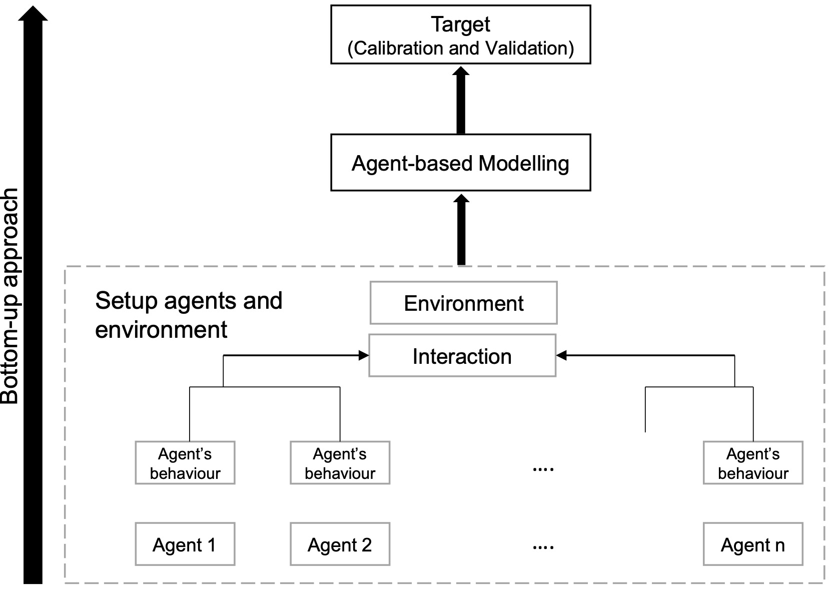
Figure 4: Framework for Agent-based modelling.
Despite these limitations and challenges, agent-based modelling has been used extensively to model infectious disease transmission and forecasting (Tracy, Cerdá, & Keyes, 2018; Venkatramanan et al., 2018). Agent-based modelling approaches have been widely used in early phases of the COVID-19 outbreak, to assess the impact of different interventions on disease spread and forecasts (Wallentin, Kaziyeva, & Reibersdorfer-Adelsberger, 2020). In a review paper, Weron (2014) states some applications of agent-based models for electricity demand forecasting. Xiao & Han (2016) use agent-based models to forecast new product diffusion. Furthermore, thinking the other way around, Hassan, Arroyo, Galán Ordax, Antunes, & Pavón Mestras (2013) explain how forecasting principles can be applied in agent-based modelling.
2.7.4 Feature-based time series forecasting51
A time series feature can be any statistical representation of time series characteristics. A vast majority of time series mining tasks are based on similarity quantification using their feature representations, including but not limited to time series clustering (Kang, Belušić, & Smith-Miles, 2014, 2015 and §2.7.12; Wang, Smith-Miles, & Hyndman, 2006), classification (Fulcher, Little, & Jones, 2013; Nanopoulos, Alcock, & Manolopoulos, 2001), anomaly detection (Kang, 2012; Talagala et al., 2020a and §2.2.3), and forecasting (Kang, Hyndman, & Smith-Miles, 2017; Montero-Manso et al., 2020 see also §2.2.5). The choice of features depends on the nature of the data and the application context. The state-of-the-art time series feature representation methods quantify a wide range of time series characteristics, including simple summary statistics, stationarity (Montero-Manso et al., 2020; Xiaoqian Wang et al., 2021), model fits (Christ, Braun, Neuffer, & Kempa-Liehr, 2018; Fulcher & Jones, 2014), time series imaging (X. Li et al., 2020b), and others. In the forecasting community, two lines of forecasting approaches have been developed using time series features, namely feature-based model selection and feature-based model combination. The motivation behind them is no single model always performs the best for all time series. Instead of choosing one model for all the data, features can be used to obtain the most appropriate model or the optimal combination of candidate models, per series.
As early as in 1972, Reid (1972) argues that time series characteristics provide valuable information in forecast model selection, which is further echoed by Makridakis & Hibon (1979). One way to forecast an extensive collection of time series is to select the most appropriate method per series according to its features. Pioneer studies focus on rule-based methods (for example, Arinze, 1994; Xiaozhe Wang et al., 2009) to recommend the “best” forecasting model per series based on its features. Another line of approaches apply regression to study how useful features are in predicting which forecasting method performs best (for example, Meade, 2000; Petropoulos et al., 2014). With the advancement of machine learning (see also §2.7.10), more recent literature uses “meta-learning” to describe the process of automatically acquiring knowledge for forecast model selection. The first such study is by Prudêncio & Ludermir (2004), who apply decision trees for forecast model selection. Lemke & Gabrys (2010) compare different meta-learning approaches to investigate which model works best in which situation. Kang et al. (2017) propose using feature spaces to visualise the strengths and weaknesses of different forecasting methods. Other algorithms such as neural networks (see also §2.7.8) and random forecasts are also applied to forecast model selection (Kück, Crone, & Freitag, 2016; Talagala, Hyndman, & Athanasopoulos, 2018).
One of the pioneering studies in feature-based forecast combination is the rule-based approach by Collopy & Armstrong (1992), who develop 99 rules for forecast combination based on 18 features. Recently, Kang et al. (2020) use 26 features to predict the performances of nine forecasting methods with nonlinear regression models, and obtain the combination weights as a tailored softmax function of the predicted forecasting errors. The feature-based forecast model averaging (FFORMA) framework proposed by Montero-Manso et al. (2020) employ 42 features to estimate the optimal combination weights of nine forecasting methods based on extreme gradient boosting (XGBoost, Chen & Guestrin, 2016). Li et al. (2020b) first transform time series into images, and use features extracted from images to estimate the optimal combination weights. For feature-based interval forecasting, Wang et al. (2021) investigate how time series features affect the relative performances of prediction intervals from different methods, and propose a general feature-based interval forecasting framework to provide reliable forecasts and their uncertainty estimation.
2.7.5 Forecasting with bootstrap52
The bootstrap methodology has been widely applied in many areas of research, including time series analysis. The bootstrap procedure Efron (1979) is a very popular methodology for independent data because of its simplicity and nice properties. It is a computer-intensive method that presents solutions in situations where the traditional methods fail or are very difficult to apply. However, Efron’s bootstrap (iid bootstrap) has revealed itself inefficient in the context of dependent data, such as in the case of time series, where the dependence structure arrangement has to be kept during the resampling scheme.
Most of the resampling for dependent data consider segments of the data to define blocks, such that the dependence structure within each block can be kept. Different versions of blocking differ in the way as blocks are constructed: the nonoverlapping block bootstrap (Carlstein, 1990), the moving block bootstrap (Künsch, 1989), the circular block bootstrap (Politis & Romano, 1992), and the stationary block bootstrap (Politis & Romano, 1994). But, if the time series process is driven from iid innovations, another way of resampling can be used.
The iid Bootstrap can then be easily extended to a dependent setup. That was the spirit of sieve bootstrap proposed by (Bühlmann, 1997). This method is based on the idea of fitting parametric models first and resampling from the residuals. Such models include, for example, the linear regression (Freedman, 1981) and autoregressive time series (Efron & Tibshirani, 1986). This approach is different from the previous bootstrap methods for dependent data; the sample bootstrap is (conditionally) stationary and does not present a structure of dependence. Another different feature is that the sieve bootstrap sample is not a subsample from the original data, as in the previous methods. Observe that even if the sieve bootstrap is based on a parametric model, it is nonparametric in its spirit. The AR model (see §2.3.4) here is just used to filter the residuals series.
A few years ago, the sieve bootstrap was used for estimating forecast intervals (Andrés, Peña, & Romo, 2002; Zagdański, 2001). Motivated by these works, Cordeiro & Neves (2006, 2009, 2010) developed a procedure to estimate point forecasts. The idea of these authors was to fit an exponential smoothing model (see §2.3.1) to the time series, extract the residuals and then apply the sieve bootstrap to the residuals. Further developments of this procedure include the estimation of forecast intervals (Cordeiro & Neves, 2014) and also the detection, estimation and imputation of missing data (Cordeiro & Neves, 2013). In a recent work (Bergmeir et al., 2016) a similar approach was also consider, the residuals were extracted and resampled using moving block bootstrap (see §2.7.6 for further discussion).
Peter J Bickel & Freedman (1981) and later in Angus (1992) showed that in extreme value theory, the bootstrap version for the maximum (or minimum) does not converge to the extremal limit laws. Zelterman (1993) pointed out that “to resample the data for approximating the distribution of the \(k\) largest observations would not work because the ‘pseudo-samples’ would never have values greater than \(X_{n:n}\)”53. A method considering to resample a smaller size than the original sample was proposed in Hall (1990). Recently, Neves & Cordeiro (2020) used this idea and developed a preliminary work in modelling and forecasting extremes in time series.
2.7.6 Bagging for time series forecasting54
The term bagging was proposed by Breiman (1996) to describe the generation of several versions of a predictor, via Bootstrap procedures (introduced in §2.7.5), with a final aggregation stage. Thus, “bootstrap aggregating” was established as bagging. The main idea is to improve predictors’ accuracy once the data sets, draw randomly with replacement, will approximating the original distribution. The author argues that bagging works for unstable procedures, but it was not tested for time series. Years after, Kilian & Inoue (2004) suggested the first attempts for temporal dependent data. For data-driven methods, to forecasting and simulation time series and deal with predictors ensembles, bagging has shown as a powerful tool.
A general framework for ensemble forecasting methods involves four main stages: (i) data treatment, (ii) resampling, (iii) forecasting, and (iv) aggregation. However, for time series, bootstrap should be done carefully, as the serial dependence and non-stationarity must be considered.
As mentioned in §2.7.5, this led Bergmeir et al. (2016) to propose a bagging version for exponential smoothing, the Bagged ETS. As pre-treatment, after a Box-Cox transformation, the series is decomposed into trend, seasonal, and remainder components via STL decomposition (Cleveland et al., 1990). The resampling stage uses moving block bootstrap (MBB: Lahiri & Lahiri, 2003), applied to the remainder. There are several discussions in the literature about this procedure, mainly regarding the size of the blocks. MBB resampling the collection of overlapping (consecutive) blocks of observations. The idea is to keep the structure still present in the remainder. The forecasts are obtained via ETS methods (see §2.3.1) and, for the final aggregation, the authors adopted the median. Their method is evaluated on the M3 data set and outperformed the original benchmarks. The work of Bergmeir et al. (2016) inspired many others: Dantas, Cyrino Oliveira, & Varela Repolho (2017) applied the idea for air transport demand data and Oliveira & Cyrino Oliveira (2018) for energy consumption, proposing the so-called remainder sieve bootstrap (RSB).
Dantas & Cyrino Oliveira (2018) proposed an extension to the Bagged ETS where bagging and exponential smoothing are combined with clustering methods (clustering-based forecasting methods are discussed in §2.7.12). The approach aims to consider and reduce the covariance effects among the ensemble time series, creating clusters of similar forecasts – since it could impact the variance of the group. A variety of forecasts are selected from each cluster, producing groups with reduced variance.
In light of the aforementioned, there are several possibilities for each stage of the mentioned framework. In this context, to investigate the reasons why bagging works well for time series forecasting, Petropoulos et al. (2018a) explored three sources of uncertainty: model form, data, and parameter. While arguably bagging can handle all of them, Petropoulos et al. (2018a) showed that simply tackling model uncertainty is enough for achieving a superior performance, leading to the proposal of a Bootstrap Model Combination (BMC) approach, where different model forms are identified in the ensemble and fitted to the original data.
Finally, Meira, Cyrino Oliveira, & Jeon (2020) proposed “treating and pruning” strategies to improve the performance of prediction intervals for both model selection and forecast combinations. Testing over a large set of real time series from the M forecasting competitions (see also §2.12.7), their results highlighted the importance of analysing the prediction intervals of the ensemble series before the final aggregation.
2.7.7 Multi-step ahead forecasting55
Given a univariate time series comprising \(n\) observations, \(y_1, y_2,\dots, y_n\), multi-step ahead point forecasting involves producing point estimates of the \(H\) future values \(y_{n+1}, y_{n+2},\dots, y_{n+H}\), where \(H > 1\), is the forecast horizon (Ben Taieb, 2014).
The (naive) recursive strategy estimates a one-step-ahead autoregressive model to predict \(y_{t+1}\) from \(y_t, y_{t-1}, \dots\), by minimising the one-step-ahead forecast errors. Each forecast is then obtained dynamically by iterating the model \(H\) times, and by plugging in the missing lagged values with their respective forecasts. The direct strategy builds separate \(h\)-step-ahead models to predict \(y_{t+h}\) from \(y_t, y_{t-1}, ...\) for \(h = 1, 2, \dots, H\), by minimising \(h\)-step-ahead forecast errors, and forecasts are computed directly by the estimated models.
In theory, with linear models, model misspecification plays an important role in the relative performance between the recursive and direct strategy (Chevillon, 2007). If the model is correctly specified, the recursive strategy benefits from more efficient parameter estimates, while the direct strategy is more robust to model misspecification. With nonlinear models, recursive forecasts are known to be asymptotically biased (Fan & Yao, 2005; J. L. Lin & Granger, 1994; Teräsvirta, Tjostheim, & Granger, 2010), and the direct strategy is often preferred over the recursive strategy since it avoids the accumulation of forecast errors. In practice, the results are mixed (Atiya, El-shoura, Shaheen, & El-sherif, 1999; Kline, 2004; Marcellino, Stock, & Watson, 2006; Pesaran, Pick, & Timmermann, 2011; Sorjamaa, Hao, Reyhani, Ji, & Lendasse, 2007), and depend on many interacting factors including the model complexity (see also §2.5.2), the (unknown) underlying data generating process, the number of observations, and the forecast horizon (see also §2.7.4).
Hybrids and variants of both recursive and direct strategies have been proposed in the literature. For example, one of the hybrid strategies (Sorjamaa & Lendasse, 2006; Zhang, Zhou, Chang, Yang, & Li, 2013; Zhang & Hutchinson, 1994) first produce recursive forecasts, then adjust these forecasts by modelling the multi-step forecast errors using a direct strategy (Ben Taieb & Hyndman, 2014). Variants of the recursive strategy match the model estimation and forecasting loss functions by minimising the implied \(h\)-step-ahead recursive forecast errors (Bhansali & Kokoszka, 2002; Bontempi, Birattari, & Bersini, 1999; McNames, 1998). Variants of the direct strategy exploit the fact that the errors of different models are serially correlated (Chen, Yang, & Hafner, 2004; Franses & Legerstee, 2009a; Lee & Billings, 2003; Pesaran et al., 2011). The idea is to reduce the forecast variance of independently selected models by exploiting the relatedness between the forecasting tasks, as in multi-task learning (Caruana, 1997). For example, a multi-horizon strategy will measure forecast accuracy (see §2.12.2) by averaging the forecast errors over multiple forecast horizons (Bontempi & Ben Taieb, 2011; Kline, 2004). Different multi-horizon strategies can be specified, with different formulation of the objective function (Ben Taieb, Sorjamaa, & Bontempi, 2010). One particular case is the multi-output strategy which estimates a single model for all horizons by minimising the average forecast error over the entire forecast horizon (Bontempi & Ben Taieb, 2011).
Forecasting strategies are often model-dependent, especially with machine learning models (see §2.7.10). Furthermore, model architecture and parameters are often trained by taking into account the chosen forecasting strategy. For example, we can naturally implement and train recursive forecasting models using recurrent neural networks (see also §2.7.8). Also, different specifications of the decoder in sequence-to-sequence models will induce different forecasting strategies, including variants of direct and multi-horizon strategies. For more details, we refer the reader to Hewamalage, Bergmeir, & Bandara (2021) and Section 4.2 in Benidis et al. (2020).
Which forecasting strategy is best is an empirical question since it involves a tradeoff between forecast bias and variance (Ben Taieb & Atiya, 2015; Ben Taieb, Bontempi, Atiya, & Sorjamaa, 2012). Therefore, the forecasting strategy should be part of the design choices and the model selection procedure of any multi-step-ahead forecasting model.
2.7.8 Neural networks56
Neural Networks (NNs) or Artificial Neural Networks (ANNs) are mathematical formulations inspired by the work and functioning of biological neurons. They are characterized by their ability to model non-stationary, nonlinear and high complex datasets. This property along with the increased computational power have put NNs in the frontline of research in most fields of science (De Gooijer & Hyndman, 2006; Zhang, Eddy Patuwo, & Y. Hu, 1998).
A typical NN topology is consisted by three types of layers (input, hidden and output) and each layer is consisted by nodes. The first layer in every NN, is the input layer and the number of its nodes corresponds to the number of explanatory variables (inputs). The last layer is the output layer and the number of nodes corresponds to the number of response variables (forecasts). Between the input and the output layer, there is one or more hidden layers where the nodes define the amount of complexity the model is capable of fitting. Most NN topologies in the input and the first hidden layer contain an extra node, called the bias node. The bias node has a fixed value of one and serves a function similar to the intercept in traditional regression models. Each node in one layer has connections (weights) with all or a subset (for example, for the convolutional neural network topology) of the nodes of the next layer.
NNs process the information as follows: the input nodes contain the explanatory variables. These variables are weighted by the connections between the input and the first hidden nodes, and the information reaches to the hidden nodes as a weighted sum of the inputs. In the hidden nodes, there is usually a non-linear function (such as the sigmoid or the RelU) which transform the information received. This process is repeated until the information reaches the output layer as forecasts. NNs are trained by adjusting the weights that connect the nodes in a way that the network maps the input value of the training data to the corresponding output value. This mapping is based on a loss function, the choice of which depends on the nature of the forecasting problem. The most common NN procedure, is the back-propagation of errors (for additional details on training, see §2.7.11).
The simpler and most common NN topology, is the Multilayer Forward Perceptron (MLP). In MLP, the hidden nodes contain the sigmoid function and the information moves in forward direction (from the inputs to the output nodes). An another NN topology where the information moves also only in a forward direction is the Radial Basis Function NN (RBF). Now the hidden neurons compute the Euclidean distance of the test case from the neuron’s centre point and then applies the Gaussian function to this distance using the spread values. Recurrent Neural Networks (RNNs) are NN topologies that allow previous outputs to be used as inputs while having hidden states. The information moves both forwards and backwards. RNNs have short-term memory and inputs are taken potentially from all previous values. MLPs, RBFs and RNNs are universal function approximators (Hornik, 1991; Park & Sandberg, 1991; Schäfer & Zimmermann, 2006). However, the amount of NN complexity in terms of hidden layers and nodes to reach this property, might make the NN topology computationally unfeasible to train (see also the discussion in §2.7.11). For the interaction of NNs with the probability theory, we refer the reader to last part of §2.7.9.
2.7.9 Deep probabilistic forecasting models57
Neural networks (§2.7.8) can be equipped to provide not only a single-valued forecast, but rather the entire range of values possible in a number of ways (see also §2.6.2 and §2.6.3). We will discuss three selected approaches in the following, but remark that this is a subjective selection and is by far not comprehensive.58
Analogously to linear regression and Generalised Linear Models, obtaining probabilistic forecasts can be achieved by the neural network outputting not the forecasted value itself but rather parameters of probability distribution or density (Bishop, 2006). In forecasting, a prominent example is the DeepAR model (Salinas et al., 2019b), which uses a recurrent neural network architecture and assumes the probability distribution to be from a standard probability density function (e.g., negative binomial or Student’s \(t\)). Variations are possible, with either non-standard output distributions in forecasting such as the multinomial distribution (Rabanser, Januschowski, Flunkert, Salinas, & Gasthaus, 2020) or via representing the probability density as cumulative distribution function (Salinas et al., 2019a) or the quantile function (Gasthaus et al., 2019).
An alternative approach is to apply concepts for quantile regression (Koenker, 2005) to neural networks, e.g., by making the neural network produce values for selected quantiles directly (Wen, Torkkola, Narayanaswamy, & Madeka, 2017).
It is possible to combine neural networks with existing probabilistic models. For example, neural networks can parametrise state space models (Durbin & Koopman, 2012) as an example for another class of approaches (Rangapuram et al., 2018), dynamic factor models (Geweke, 1977) with neural networks (Wang et al., 2019) or deep temporal point processes (Turkmen, Wang, & Januschowski, 2019).
The appeals of using neural networks for point forecasts carry over to probabilistic forecasts, so we will only comment on the elegance of modern neural network programming frameworks. To the forecasting model builder, the availability of auto gradient computation, the integration with highly-tuned optimisation algorithms and scalability considerations built into the frameworks, means that the time from model idea to experimental evaluation has never been shorter. In the examples above, we brushed over the need to have loss functions with which we estimate the parameters of the neural networks. Standard negative log-likelihood based approaches are easily expressible in code as are approaches based on non-standard losses such as the continuous ranked probability score (Gneiting et al., 2007 and §2.12.4). With open source proliferating in the deep learning community, most of the above examples for obtaining probabilistic forecasts can readily be test-driven (see, for example, Alexandrov et al., 2019).
For the future, we see a number of open challenges. Most of the approaches mentioned above are univariate, in the following sense. If we are interested in forecasting values for all time series in a panel, we may be interested in modelling the relationship among these time series. The aforementioned approaches mostly assume independence of the time series. In recent years, a number of multivariate probabilistic forecasting models have been proposed (Rangapuram, Bezenac, Benidis, Stella, & Januschowski, 2020; Salinas et al., 2019a), but much work remains to obtain a better understanding. Another counter-intuitive challenge for neural networks is to scale them down. Neural networks are highly parametrised, so in order to estimate parameters correctly, panels with lots of time series are needed. However, a large part of the forecasting problem landscape (Januschowski & Kolassa, 2019) consists of forecasting problems with only a few time series. Obtaining good uncertainty estimates with neural networks in these settings is an open problem.
2.7.10 Machine learning59
Categorising forecasting methods into statistical and machine learning (ML) is not trivial, as various criteria can be considered for performing this task (Januschowski et al., 2020). Nevertheless, more often than not, forecasting methods are categorised as ML when they do not prescribe the data-generating process, e.g., through a set of equations, thus allowing for data relationships to be automatically learned (Barker, 2020). In this respect, methods that build on unstructured, non-linear regression algorithms (see also §2.3.2), such as Neural Networks (NN), Decision Trees, Support Vector Machines (SVM), and Gaussian Processes, are considered as ML (Makridakis, 2018).
Since ML methods are data-driven, they are more generic and easier to be adapted to forecast series of different characteristics (Spiliotis et al., 2020b). However, ML methods also display some limitations. First, in order for ML methods to take full advantage of their capacity, sufficient data are required. Thus, when series are relatively short and display complex patterns, such as seasonality and trend, ML methods are expected to provide sub-optimal forecasts if the data are not properly pre-processed (Makridakis, 2018; Zhang et al., 1998). On the other hand, when dealing with long, high-frequency series, typically found in energy (Chae, Horesh, Hwang, & Lee, 2016 but also §3.4), stock market (Moghaddam, Moghaddam, & Esfandyari, 2016 and §3.3), and demand (Carmo & Rodrigues, 2004 but also §3.2) related applications, ML methods can be applied with success. Second, computational intensity may become relevant (Makridakis et al., 2020b), especially when forecasting numerous series at the weekly and daily frequency (Seaman, 2018) or long-term accuracy improvements over traditional methods are insignificant (Nikolopoulos & Petropoulos, 2018). Third, given that the effective implementation of ML methods strongly depends on optimally determining the values of several hyper-parameters, related both with the forecasting method itself and the training process, considerable complexity is introduced, significant resources are required to set up the methods, and high experience and a strong background in other fields than forecasting, such as programming and optimisation, are needed.
In order to deal with these limitations, ML methods can be applied in a cross-learning (CL) fashion instead of a series-by-series one (Makridakis et al., 2020b), i.e., allow the methods to learn from multiple series how to accurately forecast the individual ones (see also §2.12.7). The key principle behind CL is that, although series may differ, common patterns may occur among them, especially when data are structured in a hierarchical way and additional information, such as categorical attributes and exogenous/explanatory variables (see §2.2.5), is provided as input (Fry & Brundage, 2020). The CL approach has several advantages. First, computational time can be significantly reduced as a single model can be used to forecast multiple series simultaneously (Semenoglou, Spiliotis, Makridakis, & Assimakopoulos, 2021). Second, methods trained in a particular dataset can be effectively used to provide forecasts for series of different datasets that display similar characteristics (transfer-learning), thus allowing the development of generalised forecasting methods (Oreshkin et al., 2020a). Third, data limitations are mitigated and valuable information can be exploited at global level, thus allowing for patterns shared among the series, such as seasonal cycles (Dekker, van Donselaar, & Ouwehand, 2004) and special events (Huber & Stuckenschmidt, 2020), to be effectively captured.
Based on the above, CL is currently considered the most effective way of applying ML for batch time series forecasting. Some state-of-the-art implementations of CL include long short-term memory NNs (Smyl, 2020), deep NNs based on backward and forward residual links (Oreshkin et al., 2020b), feature-based XGBoost (Montero-Manso et al., 2020), and gradient boosted decision trees (Bojer & Meldgaard, 2020).
2.7.11 Machine learning with (very) noisy data60
With the advent of big data, machine learning now plays a leading role in forecasting.61 There are two primary reasons for this. First, conventional ordinary least squares (OLS) estimation is highly susceptible to overfitting in the presence of a large number of regressors (or features); see also §2.5.2 and §2.5.3. OLS maximises the fit of the model over the estimation (or training) sample, which can lead to poor out-of-sample performance; in essence, OLS over-responds to noise in the data, and the problem becomes magnified as the number of features grows. A class of machine-learning techniques, which includes the popular least absolute shrinkage and selection operator (LASSO, Tibshirani, 1996) and elastic net (ENet, Zou & Hastie, 2005), employs penalised regression to improve out-of-sample performance with large numbers of features. The LASSO and ENet guard against overfitting by shrinking the parameter estimates toward zero.
Very noisy data – data with a very low signal-to-noise ratio – exacerbate the overfitting problem. In such an environment, it is vital to induce adequate shrinkage to guard against overfitting and more reliably uncover the predictive signal amidst all the noise. For LASSO and ENet estimation, a promising strategy is to employ a stringent information criterion, such as the Bayesian information criterion (BIC, Schwarz, 1978), to select (or tune) the regularisation parameter governing the degree of shrinkage (often denoted by \(\lambda\)). Hansheng Wang et al. (2009) and Fan & Tang (2013) modify the BIC penalty to account for a diverging number of features, while Hui, Warton, & Foster (2015) refine the BIC penalty to include the value of \(\lambda\). These BIC variants induce a greater degree of shrinkage by strengthening the BIC’s penalty term, making them useful for implementing the LASSO and ENet in noisy data environments; see Filippou, Rapach, Taylor, & Zhou (2020) for a recent empirical application.
A second reason for the popularity of machine learning in the era of big data is the existence of powerful tools for accommodating complex predictive relationships. In many contexts, a linear specification appears overly restrictive, as it may neglect important nonlinearities in the data that can potentially be exploited to improve forecasting performance. Neural networks (NNs; see §2.7.8) are perhaps the most popular machine-learning device for modelling nonlinear predictive relationships with a large number of features. Under a reasonable set of assumptions, a sufficiently complex NN can approximate any smooth function (for example, Cybenko, 1989; Barron, 1994; Funahashi, 1989; Hornik, Stinchcombe, & White, 1989).
By design, NNs are extremely flexible, and this flexibility means that a large number of parameters (or weights) need to be estimated, which again raises concerns about overfitting, especially with very noisy data. The weights of a NN are typically estimated via a stochastic gradient descent (SGD) algorithm, such as Adam (Kingma & Ba, 2015). The SGD algorithm itself has some regularising properties, which can be strengthened by adjusting the algorithm’s hyperparameters. We can further guard against overfitting by shrinking the weights via LASSO or ENet penalty terms, as well as imposing a dropout rate (Hinton, Srivastava, Krizhevsky, Sutskever, & Salakhutdinov, 2012; Srivastava, Hinton, Krizhevsky, Sutskever, & Salakhutdinov, 2014).
Perhaps the quintessential example of a noisy data environment is forecasting asset returns, especially at short horizons (e.g., monthly). Because many asset markets are reasonably efficient, most of the fluctuations in returns are inherently unpredictable – they reflect the arrival of new information, which, by definition, is unpredictable. This does not mean that we should not bother trying to forecast returns, as even a seemingly small degree of return predictability can be economically significant (e.g., Campbell & Thompson, 2008). Instead, it means that we need to be particularly mindful of overfitting when forecasting returns in the era of big data. §3.3.13 discusses applications of machine-learning techniques for stock return forecasting.
2.7.12 Clustering-based forecasting62
The robustness of the forecasting process depends mainly on the characteristics of the target variable. In cases of high nonlinear and volatile time series, a forecasting model may not be able to fully capture and simulate the special characteristics, a fact that may lead to poor forecasting accuracy (Pradeepkumar & Ravi, 2017). Contemporary research has proposed some approaches to increase the forecasting performance (Sardinha-Lourenço, Andrade-Campos, Antunes, & Oliveira, 2018). Clustering-based forecasting refers to the application of unsupervised machine learning in forecasting tasks. The scope is to increase the performance by employing the information of data structure and of the existing similarities among the data entries (Goia, May, & Fusai, 2010); see also §2.7.4 and §2.7.10. Clustering is a proven method in pattern recognition and data science for deriving the level of similarity of data points within a set. The outputs of a clustering algorithm are the centroids of the clusters and the cluster labels, i.e., integer numbers that denote the number of cluster that a specific data entry belongs to Xu & Wunsch (2005).
There are two approaches in clustering-based forecasting: (i) Combination of clustering and supervised machine learning, and (ii) solely application of clustering. In the first case, a clustering algorithm is used to split the training set into smaller sub-training sets. These sets contain patterns with high similarity. Then for each cluster a dedicated forecaster is applied (Chaouch, 2014; Fan, Chen, & Lee, 2008). Thus, the number of forecasting algorithms is equal to the number of clusters. This approach enables to train forecasters with more similar patterns and eventually achieve better training process. The forecasting systems that involve clustering are reported to result in lower errors (Fan, Mao, & Chen, 2006; Mori & Yuihara, 2001). The combination of clustering and forecasting has been presented in the literature earlier than the sole application of clustering. One of the first articles in the literature on combining clustering and forecasting sets up the respective theoretical framework (Kehagias & Petridis, 1997).
In the second case, a clustering algorithm is used to both cluster the load data set and perform the forecasting (López, Valero, Senabre, Aparicio, & Gabaldon, 2012). In the sole clustering applications, either the centroids of the clusters can be utilised or the labels. Pattern sequence-based forecasting is an approach that employs the cluster labels. In this approach, a clustering of all days prior to the test day is held and this results in sequences of labels of a certain length. Next, the similarity of the predicted day sequence with the historical data sequences is examined. The load curve of the predicted day is the average of the curves of the days following the same sequences (Kang, Spiliotis, et al., 2020; Martinez Alvarez, Troncoso, Riquelme, & Aguilar Ruiz, 2011).
There is variety of clustering algorithms that have been proposed in forecasting such as the \(k\)-means, fuzzy C-means (FCM), self-organising map (SOM), deterministic annealing (DA), ant colony clustering ACC, and others. Apart from the clustering effectiveness, a selection criterion for an algorithm is the complexity. \(k\)-means and FCM are less complex compared to the SOM that needs a large number of variables to be calibrated prior to its application. Meta-heuristics algorithms, such as ACC, strongly depend on the initialisation conditions and the swarm size. Therefore, a comparison of clustering algorithms should take place to define the most suitable one for the problem under study (Elangasinghe, Singhal, Dirks, Salmond, & Samarasinghe, 2014; Li, Han, & Li, 2008; Mori & Yuihara, 2001; Weina Wang et al., 2015).
The assessment of clustering-based forecasting is held via common evaluation metrics for forecasting tasks (see also §2.12). The optimal number of clusters, which is a crucial parameter of a clustering application, is selected via trial-and-error, i.e., the optimal number corresponds to the lowest forecasting error (Nagi, Yap, Nagi, Tiong, & Ahmed, 2011).
2.7.13 Hybrid methods63
Hybrid approaches combine two or more of the above-mentioned advanced methods. In general, when methods based on AI-based techniques, physical, and statistical approaches are combined together, the result is often improved forecasting accuracy as a benefit from the inherent integration of the single methods. The idea is to mix diverse methods with unique features to address the limitations of individual techniques, thus enhancing the forecast performance (Mandal, Madhira, Haque, Meng, & Pineda, 2012 see also §2.6; Nespoli et al., 2019). The performance of the hybrid methods depends on the performance of the single methods, and these single methods should be specifically selected for the problem that has to be addressed.
Hybrid methods can be categorised based on the constituent methods, but also considering that these base methods may not necessarily act only on the forecasting stage but also on data treatment and parameters identification stages. In data pre-processing combining approaches (see also §2.2), different methods can be used for decomposing the time series into subseries (Son, Yang, & Na, 2019) or the signal into different frequencies (Zang et al., 2018), and for classifying the historical data (C. Huang et al., 2015). An advantage of such hybrid methods is robustness against sudden changes in the values of the main parameters. However, they require additional knowledge and understanding of the base methods, and have the disadvantage of slow response time to new data.
The purpose of the parameter selection stage is to optimise the parameters of the model, in terms of extracting nonlinear features and invariant structures (Behera, Majumder, & Nayak, 2018; Ogliari, Niccolai, Leva, & Zich, 2018) but also in terms of estimation of the parameter adopted for the prediction; for example, meteorological factors such as temperature, humidity, precipitation, snowfall, cloud, sunshine, wind speed, and wind direction (Qu, Kang, Zhang, Jiang, & Ma, 2016). Hybrid methods feature straightforward determination of the parameters with relatively basic structures. However, the implementation is sometimes challenging, and depends on the knowledge and expertise of the designer.
Finally, the data post-processing hybrid approaches forecast the residual errors resulted from the forecasting model. Since these hybrid methods consider residual errors from the model, they aim in further improving the predictions of the base methods by applying corrections in the forecasts. However, a disadvantage of these hybrid methods is the increased calculation time, as the residual errors must also be estimated. Also, such hybrid methods are not general and will depend on the field of application. In many cases, hybrids approaches outperform other (single) approaches such as \(k\)NN, NN, and ARIMA-based models (Mellit, Massi Pavan, Ogliari, Leva, & Lughi, 2020). A great example is the hybrid method by Smyl (2020), which achieved the best performance in the M4 forecasting competition (see also §2.12.7). In particular, in energy applications (see §3.4), a combination of physical and AI-based techniques can lead to improved forecasting performance. Furthermore, machine learning methods (see §2.7.10) based on historical data of meteorological variables combined with an optimal learning algorithm and weather classification can further improve the forecasting accuracy of single methods. However, in general, the weak point of such hybrid approaches is that they underperform when meteorological conditions are unstable (Chicco, Cocina, Di Leo, Spertino, & Massi Pavan, 2015).
2.8 Methods for intermittent demand
2.8.1 Parametric methods for intermittent demand forecasting64
Demand forecasting is the basis for most planning and control activities in any organisation. Demand will typically be accumulated in some pre-defined ‘time buckets’ (periods), such as a day, a week or a month. On many occasions, demand may be observed in every time period, resulting in what is sometimes referred to as ‘non-intermittent demand’. Alternatively, demand may appear sporadically, with no demand at all in some periods, leading to an intermittent appearance of demand occurrences. Intermittent demand items monopolise the stock bases in the after sales industry and are prevalent in many other industries, including the automotive, IT, and electronics sectors. Their inventory implications are dramatic and forecasting their requirements is a very challenging task.
Methods to forecast intermittent demand may broadly be classified as parametric and non-parametric. The former suppose that future demand can be well represented by a statistical distribution (say Poisson or Negative Binomial) which has parameters that are unknown but may be forecasted using past data. These methods are discussed in this sub-section. In the latter, the data are not assumed to follow any standard probability distribution. Instead, direct methods are used to assess the distributions required for inventory management (see also §3.2.3). Such methods are discussed in §2.8.2.
Simple Exponential Smoothing (SES; see §2.3.1) is often used in practice to forecast intermittent demand series. However, SES fails to recognise that intermittent demand is built from two constituent elements: (i) the inter-demand intervals, which relate to the probability of demand occurring, and (ii) the demand sizes, when demand occurs. The former indicates the degree of intermittence, whereas the latter relates to the behaviour of the positive demands. Croston (1972) showed that this inherent limitation leads to SES being (positively) biased after a demand occurring period; this is sometimes referred to as an ‘issue point’ bias. Subsequently, he proposed a method that forecasts separately the sizes of demand, when demand occurs, and the inter-demand intervals. Both forecasts are produced using SES, and the ratio of the former over the latter gives a forecast of the mean demand per period. Croston’s method was shown by Syntetos & Boylan (2001) to suffer from another type of bias (inversion bias) and the same researchers Aris A Syntetos & Boylan (2005) proposed a modification to his method that leads to approximately unbiased estimates. This method is known in the literature as the Syntetos-Boylan Approximation (SBA). It has been found repeatedly to account for considerable empirical inventory forecasting improvements (Eaves & Kingsman, 2004; Gutierrez, Solis, & Mukhopadhyay, 2008; Nikolopoulos, Babai, & Bozos, 2016; Wingerden, Basten, Dekker, & Rustenburg, 2014) and, at the time of writing, it constitutes the benchmark against which other (new) proposed methodologies in the area of intermittent demand forecasting are assessed.
Croston’s method is based upon the assumption of a Bernoulli demand arrival process. Alternatively, demand may be assumed to arrive according to a Poisson process. It is also possible to adapt Croston’s method so that sizes and intervals are updated based on a simple moving average (SMA) procedure instead of SES. Boylan & Syntetos (2003), Shale, Boylan, & Johnston (2006), and Aris A Syntetos et al. (2015a) presented correction factors to overcome the bias associated with Croston’s approach under a Poisson demand arrival process and/or estimation of demand sizes and intervals using an SMA.
For a detailed review of developments in intermittent demand forecasting interested readers are referred to Boylan & Syntetos (2021).
2.8.2 Non-parametric intermittent demand methods65
Two main non-parametric forecasting approaches have dominated the intermittent demand literature: the bootstrapping approach and the Overlapping/Non-Overlapping aggregation Blocks approach (Boylan & Syntetos, 2021).
The bootstrapping approach relies upon a resampling (with or without replacement) of the historical demand data to build the empirical distribution of the demand over a specified interval. As discussed in §2.7.5, this approach was initially introduced by Efron (1979). Since then, it has been developed by Willemain, Smart, & Schwarz (2004) and Zhou & Viswanathan (2011) to deal with intermittent demand items (Babai, Tsadiras, & Papadopoulos, 2020). Willemain et al. (2004) have proposed a method that resamples demand data by using a Markov chain to switch between no demand and demand periods. The empirical outperformance of this method has been shown when compared to Simple Exponential Smoothing (SES) and Croston’s method (see also §2.8.1). However, the findings of Willemain et al. (2004)’s work have been challenged by Gardner & Koehler (2005) and some limitations have been addressed by Aris A Syntetos et al. (2015b). Zhou & Viswanathan (2011) have developed an alternative bootstrapping method. Their method samples separately demand intervals and demand sizes and it has been shown to be associated with a good performance for long lead-times. Teunter & Duncan (2009) and Hasni et al. (2019a) have developed adjustments of the bootstrapping methods, where the lead-time demand forecast is adjusted by assuming that the first period in the lead-time bucket corresponds to a non-zero demand. They have demonstrated the outperformance of the adjusted bootstrapping methods in a periodic order-up-to-level inventory control system. A review of the bootstrapping methods in the context of intermittent demand is provided by Hasni et al. (2019b).
Porras & Dekker (2008) were the first to consider aggregation with overlapping and non-overlapping blocks (OB and NOB) approach in forecasting the demand of spare parts. In the NOB approach, a demand series is divided into consecutive non-overlapping blocks of time, whereas in OB, at each period the oldest observation is dropped and the newest is included (Rostami-Tabar, Babai, Syntetos, & Ducq, 2013). Boylan & Babai (2016) have compared the statistical and inventory performance of the OB and NOB methods. They found that, unless the demand history is short, there is a clear advantage of using OB instead of NOB. More recently, based on extreme value theory (EVT), Zhu, Dekker, Jaarsveld, Renjie, & Koning (2017) have proposed an improvement of the OB method that models better the tail of lead-time demand. They have shown that the empirical-EVT method leads to higher achieved target cycle service levels when compared to the original method proposed by Porras & Dekker (2008). Temporal aggregation is further discussed in §2.10.2.
2.8.3 Classification methods66
In many application areas, forecasts are required across a wide collection of products, services or locations. In this situation, it is convenient to introduce classification rules that allow subsets of time series to be forecasted using the same approaches and methods. Categorisation rules, such as the ABC inventory classification, serve the forecasting function only coincidentally. They do not necessarily align to the selection of the best forecasting method.
Within certain modelling frameworks, classification of time series is well established. For example, within an ARIMA framework (Box, Jenkins, & Reinsel, 2008 and §2.3.4), or within a state-space framework for exponential smoothing (Hyndman et al., 2002 and §2.3.1), series may be classified, for example based on the AIC (Akaike, 1973). It is more challenging to classify series according to their recommended forecasting method if some of the candidate methods, such as Croston’s method (see §2.8.1), lack a fully satisfactory model base. In the field of intermittent demand forecasting, A A Syntetos et al. (2005) proposed the SBC classification scheme, enabling time series to be classified according to their length of average demand interval and coefficient of variation of demand sizes (when demand occurs). These rules were based on assumptions of independent and identically distributed (iid) demand, and a comparison of expected mean square error between methods. The scheme has been extended by Kostenko & Hyndman (2006) and by Petropoulos & Kourentzes (2015). In an empirical case-study, Boylan, Syntetos, & Karakostas (2008) examined series not necessarily conforming to iid assumptions and found the rules to be robust to inexact specification of cut-off values. Moon, Simpson, & Hicks (2013) used logistic regression to classify time series of demand for spare parts in the South Korean Navy. The classification was designed to identify superior performance (accuracy and inventory costs) of direct and hierarchical forecasting methods, based on the serial correlation of demands, the coefficient of variation of demand volume of spare parts (see also §3.2.7), and the functionality of the naval equipment.
Bartezzaghi, Verganti, & Zotteri (1999) identified five factors that contribute towards intermittence and ‘lumpiness’ (intermittence with highly variable demand sizes): number of potential customers, frequency of customers’ requests, heterogeneity of customers, variety of individual customer’s requests, and correlations between customers’ requests. These may contribute towards useful classifications, for example by the number of customers for an item. When this number is low and some of the customers are large, then direct communication with the customers can inform judgmental forecasts. Similarly, if a customer’s requests are highly variable, then ‘advance demand information’ from customers can help to improve judgmental estimates. These strategies can be very useful in a business-to-business environment, where such strategies are feasible.
An alternative approach to classification is combination of forecasts (see §2.6 for a review, and §2.6.1 in particular). Petropoulos & Kourentzes (2015) investigated combining standard forecasting methods for intermittent demand (e.g., SES, Croston, Syntetos-Boylan Approximation; see also §2.8.1). They did not find this to improve accuracy directly, but obtained good results from the use of combinations of forecasts at different temporal frequencies, using methods selected from the extended SBC classification scheme.
2.8.4 Peak over the threshold67
In the forecasting literature, Nikolopoulos (2020) argues that great attention has been given to modelling fast-moving time series with or without cues of information available (Nikolopoulos, Goodwin, Patelis, & Assimakopoulos, 2007). Less attention has been given to intermittent/count series (see §2.8.1, §2.8.2, and §2.3.8), which are more difficult to forecast given the presence of two sources of uncertainty: demand volume, and timing.
Historically there have been few forecasting methods developed specifically for such data (Syntetos et al., 2015b). We believe that through a time series decomposition approach á la (Leadbetter, 1991) we can isolate ‘peaks over threshold’ (POT) data points, and create new intermittent series from any time series of interest. The derived series present almost identical characteristics with the series that Croston (1972) analysed. In essence one could use such decomposition forecasting techniques to tackle much more difficult phenomena and problems coming from finance, politics, healthcare, humanitarian logistics, business, economics, and social sciences.
Any time series can be decomposed into two sub-series: one containing the baseline (white swans) and one containing the extreme values over an arbitrary-set or rule-based-set threshold (grey and black swans) as proposed by Taleb (2008); see also §2.3.22. Unfortunately, major decision-related risks and most of the underlying uncertainty lay with these extremes. So, it is very important to be able to effectively model and forecast them.
It is unlikely that any forecasting approach will accurately give the exact timing of the forthcoming extreme event, but it will instead provide a satisfactory cumulative forecast over a long period of time. The question still stands what can one do with this forecast? For earthquake data, although even if we know that a major earthquake is going to hit a region, it is almost impossible to decide to evacuate cities, but still we can influence and legislate the way structures are built and increase the awareness, training, preparedness and readiness of the public; and also ensure enough capital on hold to cope with the aftermath of the major event. For epidemics/pandemics (see §3.6.2) there are clear implications, as we have evidenced with COVID-19, on how proactively we can source and secure human resources, medical supplies, etc.
What is the current doctrine when forecasting in such a context: advanced probabilistic models. These methods typically require a lot of data and reconstruct the distributions of the underlying phenomena. These come with common successes and a plethora of constraints: big data sets needed for training the models, high mathematical complexity, and invisibility to practitioners how these methods do actually work and thus less acceptance in practice. Yet again, forecasting accuracy is the name of the game and thus these forecasting methods are serious contenders for the task in hand.
Extreme Value Theory (EVT) analyses extreme deviations from statistical measures of central location to estimate the probability of events that are more extreme than anything observed in the time series. This is usually done in the following two ways (Nikolopoulos, 2020): (i) deriving maxima and/or minima series as a first step and then having the Generalised Extreme Value Distribution fitted (often the number of extreme events is limited), and (ii) isolating the values that exceed a threshold (point over threshold) that can also lead to only a few instances extracted – so a very intermittent series in nature. The analysis involves fitting a Poisson distribution for the number of events in a basic time period and a second distribution – usually a Generalised Pareto Distribution – for the size of the resulting POT values.
2.9 Reasoning and mining
2.9.1 Fuzzy logic68
The “classical” Boolean logic is not able to handle for uncertainties and/or vagueness that are necessary when dealing with many real world problems. This is in part due to the fact that the Boolean logic is based on only two values (i.e., a statement can only be true or false). Fuzzy logic tries to overcome this issue by admitting that a statement/variable could be partially true or partially false. Mathematically, the fuzzy logic framework is based on the work of (Zadeh, 1965) who introduced the theory of fuzzy sets. The main point of this theory is the definition of two kinds of sets:
Crisp sets are the “classical” sets in the Boolean logic. An element can belong (or not) to a certain set.
Fuzzy sets, where an element can belong to the sets with a certain membership grade, with a value that varies in the interval \([0,1]\).
The definition of the fuzzy sets allows the framework to take into account the uncertainty and vagueness of information. An extension of this approach is related to the fact that a certain variable can assume a crisp value (classical theory) or can belong to different fuzzy sets with different membership grade. For example, in a system implemented to forecast the daily pollutant concentration in atmosphere, one of the inputs could relate to the weather conditions, such as the wind speed. In the classical approach, the system must have as an input the value of the wind speed at a certain day. In the fuzzy approach, the input of the system could be the membership grade of the input variable to three different fuzzy sets: (i) “Not windy”, (ii) “average windy”, and (iii) “strong windy”. On the other hand, the user of the forecasting system may be only interested in a classification of the output variable instead of the crisp value. In this case, the fuzzy approach is applied to the pollutant concentration which could belong with a certain degree to the fuzzy sets (i) “not polluted day”, (ii) “medium polluted day”, (iii) “high polluted day”, and (iv) “critical polluted day”.
In fuzzy theory, each fuzzy set is characterised by a (generally nonlinear) function, called the membership function, linking crisp values to the membership of the different sets. The association of a crisp value to its membership for a set is called fuzzyfication, while the inverse operation (from a membership value to a crisp value) is called defuzzification. As with the logic theory, the inference system assumes a key role in the fuzzy theory. A Fuzzy Inference System (FIS) allows the interpretation of the membership grades of the input variable(s) and, given some sets of fuzzy rules, assigns the corresponding values to the output variable(s). In the literature, two main fuzzy inference systems are presented:
2.9.2 Association rule mining69
Association rule mining is an exploratory data-driven approach which is able to automatically and exhaustively extract all existing correlations in a data set of categorical features. It is a powerful but computationally intensive technique, successfully applied in different forecasting contexts (Acquaviva et al., 2015; Apiletti & Pastor, 2020; Di Corso, Cerquitelli, & Apiletti, 2018). Its results are in a human-readable form.
The data set must be in the form of transactions, i.e., a collection of events, each described by categorical features. If the phenomena under analysis are modelled by continuous-valued variables, discretisation can be applied to obtain a suitable data set.
Association rule mining core task is the frequent itemset extraction, which consists in finding frequently-occurring relationships among items in a data set (Han, Pei, & Kamber, 2011). Given a data set of records characterised by several attributes, an item refers to a pair of (attribute \(=\) value), while a set of items is called itemset. The support count of an itemset is the number of records \(r\) containing that itemset. The support of an itemset is the percentage of records containing it with respect to the total number of records in the data set. An itemset is frequent when its support is greater than or equal to a minimum support threshold.
An association rule is an implication in the form \(A \rightarrow B\), where \(A\) and \(B\) are disjoint itemsets (i.e., \(A \cap B = \emptyset\)) (Tan, Steinbach, & Kumar, 2005). \(A\) is called rule body or antecedent and \(B\) rule head or consequent.
To evaluate the quality of an association rule, the support, confidence, and lift metrics are commonly exploited (Han et al., 2011). Rule support is the fraction of records containing both \(A\) and \(B\), indicating the probability that a record contains every item in these itemsets. The support of the rule is computed as the support of the union of \(A\) and \(B\).
Rule confidence represents the strength of the implication, and is the conditional probability that a transaction containing \(A\) also contains \(B\), \(P(B|A)\), i.e., the proportion of records that contain \(A\) with respect to those that also contain \(B\).
Finally, the lift of a rule measures the correlation between antecedent and consequent. It is defined as the ratio between the rule \(A \rightarrow B\) confidence and the support of \(B\). A lift ratio equal to 1.0 implies that itemsets \(A\) and \(B\) are not correlated. A lift higher than 1.0 indicates a positive correlation, meaning that the occurrence of \(A\) likely leads to the occurrence of \(B\) with the given confidence. The greater the lift, the stronger the association. Finally, a lift lower than 1.0 indicates a negative correlation between \(A\) and \(B\).
The problem of association rule mining consists in the extraction of all the association rules having rule support and confidence greater than the respective support and confidence thresholds, \(MinConf\) and \(MinSup\), defined as parameters of the mining process (Tan et al., 2005). These thresholds allow to control the statistical relevance of the extracted rules.
The process of rule mining consists of two steps. The first step is the computation of frequent itemsets, i.e., itemsets with support greater or equal to \(MinSup\). The second step is the extraction of association rules from frequent itemsets. Let be \(F\) a frequent itemset, hence having a support higher than \(MinSup\), pairs \(A\) and \(B=F-A\) are derived so that the confidence of \(A \rightarrow B\) is higher than \(MinConf\). The first step of the process is the most computationally expensive. Thus, several algorithms have been proposed to solve the problem of frequent itemset extraction (Zaki, 2000), some specifically addressing high-dimensionality issues (Apiletti et al., 2015, 2017). Despite being computationally demanding, association rule mining is an exhaustive approach, i.e., all and only statistically relevant correlations are extracted. §3.8.11 offers an example of applying association rule mining to forecast the quality of beverages.
2.9.3 Forecasting with text information70
Text data, such as social media posts, scholar articles and company reports, often contains valuable information that can be used as predictors in forecasting models (Aggarwal & Zhai, 2012). Before extracting useful features from the data, a text document needs to be cleaned and normalised for further processing. The first step of preparing the data is to filter out stop words – the words that do not add much meaning to a sentence, e.g., “a”, “is”, and “me”. For grammatical reasons, it is necessary for documents to use different forms of words. Stemming and lemmatisation can be applied to reduce inflectional forms or relate different forms of a word to a common base form. Stemming often chops off the end of a word, while lemmatisation uses vocabularies and morphological analysis to return the base form (or the lemma) of a word (Lovins, JB, 1968; Manning, Schütze, & Raghavan, 2008). For example, the word “industries" will be turned into”industri" or “industry” if stemming or lemmatisation is applied.
To model and analyse text data, we need to transform it into numerical representations so the forecasting models can process them as predictors. One way of transforming the data is through sentiment analysis. Sentiment analysis is often applied to detect polarity within customer materials such as reviews and social media posts (Archak, Ghose, & Ipeirotis, 2011; Das & Chen, 2007). An easy way to obtain the sentiment score of a word is to look it up in a happiness dictionary (for example, the hedonometer dictionary, Hedonometer, 2020). Another common way of representing the sentiment is to use a vector of numeric values that denote the word’s positivity, negativity and neutrality based on existing lexical databases such as the WordNet (Baccianella, Esuli, & Sebastiani, 2010; Godbole, Srinivasaiah, & Skiena, 2007). Once the sentiment of each word is calculated, we can apply an aggregation algorithm (e.g., simple average) to measure the sentiment of an entire sentence or paragraph.
In scholar articles and company reports, context features might be more important than sentiments. The bag-of-words model and word embeddings are often applied to generate numeric representations of such text. A bag-of-words model simply returns a matrix that describes the occurrence of words within a document (Goldberg, 2017). When we use this matrix as input to a forecasting model, each word count can be considered as a feature. The Word2Vec method is a widely used embedding method that is built based on the context of a word. Specifically, it trains a two-layer neural network that takes each word as an input to predict its surrounding words (see §2.7.8 for a discussion of neural networks for forecasting). The weights from the input layer to the hidden layer are then utilised as the numerical representation for the input word (Le & Mikolov, 2014). Once the text is turned into numeric representations, they can be used as predictors in any forecasting models. The most challenging part in this process is to find the right technique to extract features from the text.
In terms of software implementation, the Natural Language Toolkit (NLTK) and SpaCy library in Python can be applied to remove stop words and stem or lemmatise text (Honnibal, 2015; Loper & Bird, 2002). The bag-of-words technique is also available in NLTK. A particular implementation of the Word2Vec model is available on Google code (2013). Moreover, a public data set of movie reviews that is commonly studied in literature is available from the Stanford NLP Group (2013).
2.10 Forecasting by aggregation
2.10.1 Cross-sectional hierarchical forecasting71
In many applications time series can be aggregated at several levels of aggregation based on geographic or logical reasons to form hierarchical structures. These are called hierarchical time series. In the retail industry (see also §3.2.4), for example, individual sales of products at the bottom-level of the hierarchy can be grouped in categories and families of related products at increasing aggregation levels, with the total sales of the shop or distribution centre at the top level (Oliveira & Ramos, 2019; Pennings & Dalen, 2017; Villegas & Pedregal, 2018). Similarly, cross-sectional hierarchies can be used for spatial aggregation to help model housing prices or traffic in transportation networks, or otherwise formed geographical demarcations (for example, Athanasopoulos, Ahmed, & Hyndman, 2009; Kourentzes & Athanasopoulos, 2019). The forecasts of hierarchical time series produced independently of the hierarchical structure generally will not add up according to the aggregation constrains of the hierarchy, i.e., they are not coherent. Therefore, hierarchical forecasting methods that generate coherent forecasts should be considered to allow appropriate decision-making at the different levels. Actually, by taking advantage of the relationships between the series across all levels these methods have shown to improve forecast accuracy (Athanasopoulos et al., 2009; Shang & Hyndman, 2017; Yagli, Yang, & Srinivasan, 2019). One of the main reasons behind this improved performance is that forecast reconciliation is effectively a special case of forecast combinations (Hollyman, Petropoulos, & Tipping, 2021); see also §2.6.
The most common approaches to hierarchical forecasting are bottom-up and top-down. In the bottom-up approach forecasts for each time series at the bottom-level are first produced and then these are added up to obtain forecasts for all other series at the hierarchy (Dunn, Williams, & Dechaine, 1976). Since forecasts are obtained at the bottom-level no information is lost due to aggregation. In the top-down approach forecasts for the top-level series are first generated and then these are disaggregated generally using historical proportions to obtain forecasts for the bottom-level series, which are then aggregated (Gross & Sohl, 1990). Hyndman, Ahmed, Athanasopoulos, & Shang (2011) claim that this approach introduces bias to the forecasts, however Hollyman et al. (2021) showed that it is possible to calculate unbiased top-down forecasts.
Recent research on hierarchical forecasting tackles the problem using a two-stage approach. Forecasts for the series at all levels of the hierarchy are first obtained independently without considering any aggregation constrains (we refer to these as base forecasts). Then, base forecasts are adjusted so that they become coherent (we refer to these as reconciled forecasts). This adjustment is achieved by a matrix that maps the base forecasts into new bottom-level forecasts which are then added up (Hyndman et al., 2011).
Wickramasuriya, Athanasopoulos, & Hyndman (2019) found the optimal solution for this matrix, which minimises the trace of the covariance matrix of the reconciled forecast errors (hence MinT reconciliation). This optimal solution is based on the covariance matrix of the base forecast errors which incorporates the correlation structure of the hierarchy. Wickramasuriya et al. (2019) presented several alternative estimators for this covariance matrix: (i) proportional to the identity which is optimal only when base forecast errors are uncorrelated and equivariant (referred to as OLS), (ii) proportional to the sample covariance estimator of the in-sample one-step-ahead base forecast errors with off-diagonal elements null accounts for the differences in scale between the levels of the hierarchy (referred to as WLS), (iii) proportional to the previous estimator unrestricted also accounts for the relationships between the series (referred to as MinT-Sample), and (iv) proportional to a shrinkage estimator based on the two previous estimators, parameterising the shrinkage in terms of variances and correlations, accounts for the correlation across levels (referred as MinT-Shrink). Other researchers focus on simple (equal-weighted) combinations of the forecasts produced at different hierarchical levels (Abouarghoub, Nomikos, & Petropoulos, 2018; Hollyman et al., 2021). Pritularga, Svetunkov, & Kourentzes (2021) showed that more complex reconciliation schemes result in more variability in the forecasts, due to the estimation of the elements in the covariance matrix, or the implicit combination weights. They provide approximations for the covariance matrix that balance this estimation uncertainty with the benefits of more finely tuned weights.
More recently these techniques were extended to probabilistic forecasting (Ben Taieb, Taylor, & Hyndman, 2020). When base forecasts are probabilistic forecasts characterised by elliptical distributions, Panagiotelis, Gamakumara, Athanasopoulos, & Hyndman (2020) showed that reconciled probabilistic forecasts also elliptical can be obtained analytically. When it is not reasonable to assume elliptical distributions, a non-parametric approach based on bootstrapping in-sample errors can be used.
2.10.2 Temporal aggregation72
Temporal aggregation is the transformation of a time series from one frequency to another of lower frequency. As an example, a time series of length \(n\) that is originally sampled at a monthly frequency can be transformed to a quarterly series of length \(n/3\) by using equally-sized time buckets of three periods each. It is usually applied in an non-overlapping manner, but overlapping aggregation can also be considered. The latter is preferred in the case when the original series is short, but has the disadvantage of applying lower weights on the few first and last observations of the series and introducing autocorrelations (Boylan & Babai, 2016 and §2.8.2).
Temporal aggregation is appealing as it allows to investigate the original series through different lenses. By changing the original frequency of the data, the apparent series characteristics also change. In the case of slow-moving series, temporal aggregation leads to decrease of intermittence (Nikolopoulos, Syntetos, Boylan, Petropoulos, & Assimakopoulos, 2011 see also §2.8). In the case of fast-moving series, higher levels of aggregation (i.e., lower frequencies) allow for better modelling of trend patterns, while lower aggregation levels (i.e., higher frequencies) are more suitable for capturing seasonal patterns (Kourentzes et al., 2014; Spithourakis, Petropoulos, Nikolopoulos, & Assimakopoulos, 2014).
Research has found evidence of improved forecasting performance with temporal aggregation for both slow (Nikolopoulos et al., 2011) and fast (Spithourakis, Petropoulos, Babai, Nikolopoulos, & Assimakopoulos, 2011) moving time series. This led to characterise temporal aggregation as a “self-improving mechanism”. The good performance of temporal aggregation was reconfirmed by Babai, Ali, & Nikolopoulos (2012), who focused on its utility performance rather than the forecast error. However, one challenge with single levels of aggregation is the choice of a suitable aggregation level for each series (Kourentzes, Rostami-Tabar, & Barrow, 2017).
Instead of focusing on a single aggregation level, Andrawis et al. (2011), Kourentzes et al. (2014), Petropoulos & Kourentzes (2014), and Petropoulos & Kourentzes (2015) suggested the use of multiple levels of aggregation, usually abbreviated as MTA (multiple temporal aggregation). This not only tackles the need to select a single aggregation level, but also partly addresses the issue of model uncertainty, instead of relying on model selection and parametrisation at a single aggregation level. Using this property, Kourentzes et al. (2017) showed that MTA will typically lead to more accurate forecasts, even if in theory suboptimal. Different frequencies allow for better identification of different series patterns, so it is intuitive to consider multiple temporal levels and benefit from the subsequent forecast combination across frequencies. Kourentzes & Petropoulos (2016) showed how multiple temporal aggregation can be extended to incorporate exogenous variables (see also §2.2.5). However, forecasting at a single level of aggregation can still result in better performance when the seasonal pattern is strong (Spiliotis et al., 2019b, 2020c).
Athanasopoulos et al. (2017) expressed multiple temporal aggregation within the hierarchical forecasting framework (see §2.10.1) using the term “temporal hierarchies”. Temporal hierarchies allow for the application of established hierarchical reconciliation approaches directly to the temporal dimension. Jeon, Panagiotelis, & Petropoulos (2019) show how temporal hierarchies can be used to obtain reconciled probabilistic forecasts, while Spiliotis et al. (2019b) explored empirical bias-adjustment strategies and a strategy to avoid excessive seasonal shrinkage. Nystrup, Lindström, Pinson, & Madsen (2020) proposed estimators for temporal hierarchies suitable to account for autocorrelation in the data. Finally, Kourentzes & Athanasopoulos (2020) applied temporal hierarchies on intermittent data, and showed that higher aggregation levels may offer structural information which can improve the quality of the forecasts.
2.10.3 Cross-temporal hierarchies73
In the last two subsections (§2.10.1 and §2.10.2), we saw two complimentary hierarchical structures, cross-sectional and temporal. Although the machinery behind both approaches is similar, often relying on the hierarchical framework by Hyndman et al. (2011) and Athanasopoulos et al. (2009), and work that followed from these (particularly Wickramasuriya et al., 2019), they address different forecasting problems. Cross-sectional hierarchies change the unit of analysis but are fixed in the period of analysis. For example, a manufacturer may operate using a hierarchy across products. The different nodes in the hierarchy will correspond to different products, product groups, super-groups, and so on, but will all refer to the same period, for example, a specific week. Temporal hierarchies do the opposite, where the unit of analysis is fixed, but the period is not. For example, we may look at the sales of a specific Stock Keeping Unit (SKU) at a daily, weekly, monthly, quarterly and annual levels. However, one can argue that having annual forecasts at the SKU level may not be useful. Similarly, having aggregate sales across an organisation at a weekly frequency is also of little value.
In connecting these to organisational decisions, we can observe that there is only a minority of problems that either cross-sectional or temporal hierarchies are natural, as typically decisions can differ across both the unit and the period (planning horizon) of analysis. In the latter case, both hierarchical approaches are more akin to statistical devices that can improve forecast accuracy through the use of forecast combinations, rather than satisfy the motivating argument behind hierarchical forecasting that is to provide coherent predictions for decisions at different levels of the hierarchy.
Cross-temporal hierarchies attempt to overcome this limitation, providing coherent forecasts across all units and periods of analysis, and therefore a common outlook for the future across decision-makers at different functions and levels within an organisation. The literature remains sparse on how to construct cross-temporal forecasts, as the size of the hierarchy can easily become problematic. Kourentzes & Athanasopoulos (2019) propose a heuristic approach to overcome the ensuing estimation issues. The approach works by compartmentalising the estimation. First, they obtain estimates of the cross-sectional reconciliation weights for each temporal level of the hierarchy. Then, these are combined across temporal levels, to a unique set that satisfies all coherency constraints. Using these combined weights, they obtain the reconciled bottom level forecasts, which can be aggregated as needed. Although they recognise that their approach can result in suboptimal results in terms of reconciliation errors, it guarantees coherent forecasts. Cross-temporal forecasts are more accurate than either temporal or cross-sectional hierarchical forecasts and provide a holistic view of the future across all planning levels and demarcations. Spiliotis et al. (2020c) also identify the problem, however, they do not focus on the coherency of forecasts and propose a sequential reconciliation across the two dimensions. This is shown to again be beneficial, but it does not achieve coherency. Arguably one can adapt the iterative correction algorithm by Kourentzes & Athanasopoulos (2020) to enforce coherency in this approach as well.
2.10.4 Ecological inference forecasting74
Ecological inference forecasting (EIF) aims to predict the inner-cells values of a set of contingency tables when only the margins are known. It defines a fundamental problem in disciplines such as political science, sociology and epidemiology (Salway & Wakefield, 2004). Cleave, Brown, & Payne (1995), Greiner (2007) and Pavia, Cabrer, & Sala (2009) describe other areas of application. The fundamental difficulty of EIF lies in the fact that this is a problem with more unknowns than observations, giving rise to concerns over identifiability and indeterminacy: many sets of substantively different internal cell counts are consistent with a given marginal table. To overcome this issue, a similarity hypothesis (and, sometimes, the use of covariates) is routinely assumed. The basic hypothesis considers that either conditional row (underlying) probabilities or fractions are similar (related) among contingency tables (Greiner & Quinn, 2010). The covariations among row and column margins of the different tables are then used to learn about the internal cells.
The above hypothesis is not a cure-all to the main drawback of this approach. EIF is exposed to the so-called ecological fallacy (Robinson, 1950): the presence of inconsistencies in correlations and association measures across different levels of aggregation. This is closely related to the well-known Simpson’s Paradox (Simpson, 1951). In this setting, the ecological fallacy is manifested through aggregation bias (Wakefield, 2004) due to contextual effects and/or spatial autocorrelation (Achen & Phillips Shively, 1995). This has led many authors to disqualify ecological inference forecasts (see, for example, Freedman, Klein, Ostland, & Roberts, 1998; Anselin & Tam Cho, 2002; Herron & Shotts, 2004; Tam Cho, 1998) and many others to study under which circumstances ecological inference predictions would be reliable (Firebaugh, 1978; Forcina & Pellegrino, 2019; Gelman, Park, Ansolabehere, Price, & Minnite, 2001; Renato Guseo, 2010). Despite the criticisms, many algorithms for solving the EIF problem can be found in the literature, mainly from the ecological regression and mathematical programming frameworks (some of them available in functions of the R statistical software).
The ecological regression literature has been prolific since the seminal papers of Goodman (1953, 1959) and Duncan & Davis (1953) and is undergoing a renaissance after King (1997): new methods generalised from \(2 \times 2\) tables to \(R \times C\) tables have been proposed (King, Rosen, & Tanner, 1999; Rosen, Jiang, King, & Tanner, 2001), the geographical dimension of the data is being explicitly considered (Calvo & Escolar, 2003; Puig & Ginebra, 2015), and new procedures combining aggregated and individual level data, including exit polls (see also §3.8.5), are introduced (Glynn & Wakefield, 2010; Greiner & Quinn, 2010; Klima, Schlesinger, Thurner, & Küchenhoff, 2019). See King, Tanner, & Rosen (2004) for a wide survey and Klima, Thurner, Molnar, Schlesinger, & Küchenhoff (2016) and Plescia & De Sio (2018) for an extensive evaluation of procedures. In mathematical programming exact and inequality constraints for the inner-cell values are incorporated in a natural way. Hence, this approach has shown itself to be a proper framework for generating ecological inference forecasts. The proposals from this approach can be traced back to Hawkes (1969) and Irwin & Meeter (1969). After them, some key references include McCarthy & Ryan (1977), Tziafetas (1986), Corominas, Lusa, & Dolors Calvet (2015), Romero, Pavı́a, Martı́n, & Romero (2020), and Pavía & Romero (2021). Solutions based on other strategies, for instance, entropy maximization, have been also suggested (see, for example, Johnston & Pattie, 2000; Bernardini Papalia & Fernandez Vazquez, 2020).
2.11 Forecasting with judgment
2.11.1 Judgmental forecasting75
People may use judgment alone to make forecasts or they may use it in combination with statistical methods. Here the focus is on pure judgmental forecasting (for judgmental adjustments, see §2.11.2). Different types of judgment heuristic (mental ‘rules of thumb’) can be used to make forecasts. The heuristic used depends on the nature of the information available to the forecaster (Harvey, 2007).
Consider cases where the only relevant information is held in the forecaster’s memory. For example, someone might be asked whether Manchester United or Burnley will win next week’s match. Here one memory-based heuristic that might be applicable is the recognition heuristic: if one recognises one object but not the other, then one should infer that the recognised object has higher value (Goldstein & Gigerenzer, 2002). In the above example, most people who recognise just one of the teams would be likely to make a correct forecast that Manchester United will win (Ayton, Önkal, & McReynolds, 2011). The availability heuristic is another memory-based heuristic that may be applicable: objects that are most easily brought to mind are those which are more likely. Thus, if we are asked which team is likely to come top of the premier league, we would say Manchester United if that is the one that most easily comes to mind. The availability heuristic is often effective because more likely events are encountered more often and more recently and are hence better remembered. However, it can be disrupted by, for example, greater media coverage of more unlikely (and hence more interesting) events.
Consider next cases in which forecasters possess information about values of one or more variables correlated with the variable to be forecast. For example, teachers may wish to forecast the grades of their students in a final examination on the basis of past records of various other measures. Kahneman & Tversky (1973) suggested that people use the representativeness heuristic to deal with this type of situation. Forecasters first select a variable that they think is able to represent the one that must be predicted. For example, a teacher may consider that frequency in attending voluntary revision classes represents a student’s ability in the final examination. Thus, if a student attended 15 of the 20 revision classes, they are likely to obtain 75% in the final examination.
Finally, consider situations in which people forecast future values of a variable on the basis of a record of previous values of that variable. There is some evidence that, when forecasting from time series, people use anchor-and-adjustment heuristics (Hogarth & Makridakis, 1981; Lawrence & O’Connor, 1992). For example, (i) when forecasting from an upward trended series, they anchor on the last data point and then make an upward adjustment to take the trend into account and (ii) when forecasting from an untrended series containing autocorrelation, they anchor on the last data point and make an adjustment towards the mean to take the autocorrelation into account.
Kahneman (2011) and others have divided cognitive processes into those which are intuitive (System 1) and those which are deliberative (System 2). We have discussed only intuitive processes underlying judgmental forecasting (Gigerenzer, 2007). However, they can be supplemented by deliberative (System 2) processes (Theocharis & Harvey, 2019) in some circumstances.
2.11.2 Judgmental adjustments of computer-based forecasts76
Judgmental adjustments to algorithmic computer-based forecasts can enhance accuracy by incorporating important extra information into forecasts (Fahimnia, Sanders, & Siemsen, 2020; McNees, 1990; Perera, Hurley, Fahimnia, & Reisi, 2019). However, cognitive factors (see, for example, §2.11.1), and motivational biases (see §3.2.2), can lead to the inefficient use of information (R. Fildes et al., 2019a), unwarranted adjustments and reductions in accuracy (Fildes, Goodwin, Lawrence, & Nikolopoulos, 2009; Franses & Legerstee, 2009b).
People may ‘egocentrically discount’ a computer’s forecasts when its rationale is less clear than their own reasoning (Bonaccio & Dalal, 2006). They can also be less tolerant of errors made by algorithms than those made by humans (Dietvorst, Simmons, & Massey, 2015 and §3.7.4; Önkal, Goodwin, Thomson, Gönül, & Pollock, 2009). The random errors associated with algorithmic forecasts, and the salience of rare large errors, can therefore lead to an unjustified loss of trust in computer forecasts. Adjustments may also give forecasters a sense of ownership of forecasts or be used to justify their role (Önkal & Gönül, 2005).
Computer-based forecasts are designed to filter randomness from time-series. In contrast, humans tend to perceive non-existent systematic patterns in random movements (O’Connor, Remus, & Griggs, 1993; Reimers & Harvey, 2011 and §3.7.3) and apply adjustments to reflect them. This can be exacerbated by the narrative fallacy (Taleb, 2008), where people invent stories to explain these random movements, and hindsight bias (Fischhoff, 2007), where they believe, in retrospect, that these movements were predictable. Recent random movements, and events, are particularly likely to attract undue attention, so long-run patterns identified by the computer are given insufficient weight (Bolger & Harvey, 1993). Damaging interventions are also probable when they result from political interference (Oliva & Watson, 2009) or optimism bias (Fildes et al., 2009), or when they reflect information already factored into the computer’s forecast, leading to double counting (Van den Broeke, De Baets, Vereecke, Baecke, & Vanderheyden, 2019).
How can interventions be limited to occasions when they are likely to improve accuracy? Requiring people to document reasons justifying adjustments can reduce gratuitous interventions (Goodwin, 2000b). Explaining the rationale underlying statistical forecasts also improved adjustment behaviour when series had a simple underlying pattern in a study by Goodwin & Fildes (1999). However, providing guidance on when to adjust was ineffective in an experiment conducted by Goodwin, Fildes, Lawrence, & Stephens (2011), as was a restriction preventing people from making small adjustments.
When determining the size of adjustments required, decomposing the judgment into a set of easier tasks improved accuracy in a study by Webby, O’Connor, & Edmundson (2005). Providing a database of past outcomes that occurred in circumstances analogous to those expected in the forecast period also improved adjustments in a study by Lee, Goodwin, Fildes, Nikolopoulos, & Lawrence (2007). Outcome feedback, where the forecaster is informed of the most recent outcome is unlikely to be useful since it contains noise and exacerbates the tendency to over-focus on recent events (Goodwin & Fildes, 1999; Petropoulos, Fildes, & Goodwin, 2016). However, feedback on biases in adjustments over several recent periods may improve judgments (Petropoulos, Goodwin, & Fildes, 2017). Feedback will be less useful where interventions are rare so there is insufficient data to assess performance.
The evidence for this section is largely based on laboratory-based studies of adjustment behaviour. §3.7.3 gives details of research into forecast adjustment in practice and discusses the role of forecasting support systems in improving the effectiveness of judgmental adjustments.
2.11.3 Judgmental model selection77
Forecasters – practitioners and researchers alike – use Forecast Support Systems (FSS) in order to perform their forecasting tasks. Usually, such an FSS allows the forecaster to load their historical data and they can then apply many different types of forecasting techniques to the selected data. The idea is that the forecaster selects the method which leads to highest forecast accuracy. Yet, there is no universally ‘best’ method, as it depends on the data that is being forecasted (see also §2.5.4). Thus, selection is important in achieving high accuracy. But how does this selection occur?
Research on judgmental selection of statistical forecasts is limited in quantity. Lawrence, Goodwin, & Fildes (2002) found that participants were not very adept at selecting good forecasting algorithms from a range offered to them by an FSS and had higher error than those who were presented with the optimal algorithm by an FSS. Petropoulos et al. (2018b) compared judgmental selection of forecasting algorithms with automatic selection based on predetermined information criteria. They found that judgmental selection was better than automatic selection at avoiding the ‘worst’ models, but that automatic selection was superior at choosing the ‘best’ ones. In the end, overall accuracy of judgmental selection was better than that of algorithmic selection. If their experiment had included more variation of the data (trends, fractals, different autoregressive factors) and variation of proposed models, this could possibly have led to better algorithmic than judgmental performance (Harvey, 2019). Time series that are more complex will place a higher cognitive load on judgmental selection. This was confirmed in a study by Han, Wang, Petropoulos, & Wang (2019), who used an electroencephalogram (EEG) for the comparison of judgmental forecast selection versus (judgmental) pattern identification. They found that pattern identification outperformed forecast selection, as the latter required a higher cognitive load, which in turn led to a lower forecasting accuracy.
It is likely that, in practice, judgmental selection is much more common than automatic selection. This preference for human judgment over advice from an algorithm has been shown in an experiment by Önkal et al. (2009). But how apt are forecasters in distinguishing ‘good’ models from ‘bad’ models? This was investigated by De Baets & Harvey (2020) in an experiment. People were asked to select the best performing model out of a choice of two different qualities (accuracies) of models (different combinations of good versus medium versus bad). People’s choice outperformed forecasts made by averaging the model outputs, lending credence to the views of Fifić & Gigerenzer (2014). The performance of the participants improved with a larger difference in quality between models and a lower level of noise in the data series. In a second experiment, De Baets & Harvey (2020) found that participants adjusted more towards the advice of what they perceived to be a good quality model than a medium or bad quality one.
Importantly, in selecting an algorithm and seeing it err, people are quick to abandon it. This phenomenon is known as ‘algorithm aversion’ (Dietvorst et al., 2015 see also §2.11.6) and is due to a ‘perfection schema’ we have in our heads where algorithms are concerned (Madhavan & Wiegmann, 2007). We do not expect them to ‘fail’ and thus react strongly when they do. While a model may not perform as it should for a particular dataset and may thus elicit algorithm aversion for that particular method, one should not abandon it for all datasets and future forecasts.
2.11.4 Panels of experts78
Panels of experts are often used in practice to produce judgmental forecasts (see, for example, §3.2.6 and §3.8.5). This is especially true in cases with limited available quantitative data and with the level of uncertainty being very high. In this section, three methods for eliciting judgmental forecasts from panels of experts are presented: the Delphi method, interaction groups (IG), and structured analogies (SA).
The Delphi method is centred around organising and structuring group communication (J. K. Rao et al., 2010), which aims to achieve a convergence of opinion on a specific real-world issue. It is a multiple-round survey in which experts participate anonymously to provide their forecasts and feedback (Rowe & Wright, 2001). At the end of each round, the facilitator collects and prepares statistical summaries of the panel of experts’ forecasts. These summaries are presented as feedback to the group, and may be used towards revising their forecasts. This loop continues until a consensus is reached, or the experts in the panel are not willing to revise their forecasts further. In some implementations of the Delphi method, justification of extreme positions (forecasts) is also part of the (anonymous) feedback process. The Delphi method results in a more accurate outcome in the decision-making process (Dalkey, 1969; Steurer, 2011). Rowe & Wright (2001) mentioned that, by adopting the Delphi method, groups of individuals can produce more accurate forecasts than simply using unstructured methods. A drawback of the Delphi method is the additional cost associated with the need to run multiple rounds, extending the forecasting process as well as increasing the potential drop-out rates. On the other hand, the anonymity in the Delphi method eliminates issues such as groupthink and the ‘dominant personalities’ effects (Van de Ven & Delbeco, 1971).
The IG method suggests that the members of the panel of experts actively interact and debate their points to the extent they have to reach an agreement on a common forecast (Litsiou, Polychronakis, Karami, & Nikolopoulos, 2019). Sniezek & Henry (1989) found that members of interacting groups provide more accurate judgments compared to individuals. However, there is mixed evidence about the forecasting potential of IG (Boje & Murnighan, 1982; Graefe & Armstrong, 2011; Scott Armstrong, 2006). Besides, the need for arranging and facilitating meetings for the IG makes it a less attractive option.
Another popular approach to judgmental forecasting using panels of experts is SA, which refers to the recollection of past experiences and the use analogies (Green & Armstrong, 2007). In the SA method, the facilitator assembles a panel of experts. The experts are asked to recall and provide descriptions, forecasts, and similarities/differences for cases analogous to the target situation, as well as a similarity ranking for each of these analogous cases. The facilitator gathers the lists of the analogies provided by the experts, and prepares summaries, usually using weighted averages of the recalled cases based on their similarity to the target situation (see also §2.6.4). Semi-structured analogies (sSA) have also been proposed in the literature, where the experts are asked to provide a final forecasts based on the analogous cases they recalled, which essentially reduces the load for the facilitator (Nikolopoulos, Litsa, Petropoulos, Bougioukos, & Khammash, 2015). Nikolopoulos et al. (2015) supported that the use of SA and IG could result to forecasts that are 50% more accurate compared to unstructured methods (such as unaided judgment). One common caveat of using panels of experts is the difficulty to identify who a real expert is. Engaging experts with high level of experience, and encouraging the interaction of experts are also supported by Armstrong & Green (2018).
2.11.5 Scenarios and judgmental forecasting79
Scenarios provide exhilarating narratives about conceivable futures that are likely to occur. Through such depictions they broaden the perspectives of decision makers and act as mental stimulants to think about alternatives. Scenarios enhance information sharing and provide capable tools for communication within organisations. By virtue of these merits, they have been widely used in corporate planning and strategy setting since 1960’s (Godet, 1982; Goodwin & Wright, 2010; Schoemaker, 1991; Wright & Goodwin, 1999, 2009). Even though utilisation of scenarios as decision advice to judgmental forecasting has been proposed earlier (Bunn & Salo, 1993; Schnaars & Topol, 1987), the research within this domain remained limited until recently when the interest in the subject has rekindled (Goodwin et al., 2019b; Önkal, Sayım, & Gönül, 2013; Wicke, Dhami, Önkal, & Belton, 2019).
The recent research has used behavioural experimentation to examine various features of scenarios and their interactions with judgmental adjustments (see §2.11.2) of model-based forecasts. Önkal et al. (2013) explored the ‘content’ effects of scenarios where through the narration either a bleak/negative future (a pessimistic scenario) or a bright/positive future (an optimistic scenario) was portrayed. On a demand forecasting context for mobile phones, the participants first received time-series data, model-based forecasts and then asked to generate point and interval forecasts as well as provide a confidence measure. With respect to the existence of scenarios, there were four conditions where the participants may receive: (i) no scenarios, (ii) optimistic scenarios, (iii) pessimistic scenarios, and (iv) both scenarios. Findings indicate that decision makers respond differently to optimistic and pessimistic scenarios. Receiving optimistic scenarios resulted in making larger adjustments to the model-based forecasts. At the same time, led to an increased confidence of the participants in their predictions. On the other hand, participants who received negative scenarios tend to lower their predictions the most among the four groups. An intriguing finding was the balancing effect of scenarios on the interval forecast symmetry. The lower interval bounds were adjusted upwards the most towards the centre-point of the interval (i.e., model-based predictions) when optimistic scenarios were received. Similarly, the upper bounds were adjusted downwards the most towards the centre-point of the interval in the presence of pessimistic scenarios.
The prospects of receiving a single scenario versus multiple scenarios were further explored in Goodwin et al. (2019b). The researchers investigated whether assimilation or contrast effects will occur when decision makers see optimistic (pessimistic) forecasts followed by pessimistic (optimistic) ones compared against receiving a single scenario in solitude. In case of assimilation, a scenario presenting an opposing world view with the initial one would cause adjustments in the opposite direction creating an offset effect. On the other hand, in case of contrast, the forecasts generated after the initial scenarios would be adjusted to more extremes when an opposing scenario is seen. In two experiments conducted in different contexts the researchers found resilient evidence for contrast effects taking place. Interestingly, seeing an opposing scenario also increased the confidence of the forecasters in their initial predictions.
In terms of the effects of scenario presence on the forecasting performance, however, the experimental evidence indicates the benefits are only circumstantial. Goodwin et al. (2019a) found that providing scenarios worsened forecast accuracy and shifted the resultant production order decisions further away from optimality. Despite this performance controversy, the decision makers express their fondness in receiving scenarios and belief in their merits (Goodwin et al., 2019b; Önkal et al., 2013). Therefore, we need more tailored research on scenarios and judgmental forecasting to reveal the conditions when scenarios can provide significant improvements to the forecasting accuracy.
2.11.6 Trusting model and expert forecasts80
Defined as “firm belief in the reliability, truth, and ability of someone/something” (Oxford English Dictionary), trust entails accepting vulnerability and risk (Rousseau, Sitkin, Burt, & Camerer, 1998). Given that forecasts are altered or even discarded when distrusted by users, examining trust is a central theme for both forecasting theory and practice.
Studies examining individual’s trust in model versus expert forecasts show that individuals often distrust algorithms (Burton, Stein, & Jensen, 2020; Meehl, 2013) and place higher trust on human advice (Diab, Pui, Yankelevich, & Highhouse, 2011; Eastwood, Snook, & Luther, 2012 but also §2.11.2, §2.11.3, and §3.7.4). We live in an era where we are bombarded with news about how algorithms get it wrong, ranging from COVID-19 forecasts affecting lockdown decisions to algorithmic grade predictions affecting university admissions. Individuals appear to prefer forecasts from humans over those from statistical algorithms even when those forecasts are identical (Önkal et al., 2009). Furthermore, they lose trust in algorithms quicker when they see forecast errors (Dietvorst et al., 2015; Prahl & Van Swol, 2017). Such ‘algorithm aversion’ and error intolerance is reduced when users have opportunity to adjust the forecasting outcome, irrespective of the extent of modification allowed (Dietvorst, Simmons, & Massey, 2018). Feedback appears to improve trust, with individuals placing higher trust in algorithms if they can understand them (Seong & Bisantz, 2008). Overuse of technical language may reduce understanding of the forecast/advice, in turn affecting perceptions of expertise and trustworthiness (Joiner, Leveson, & Langfield-Smith, 2002). Explanations can be helpful (Goodwin et al., 2013b), with their packaging affecting judgments of trustworthiness (Elsbach & Elofson, 2000). Algorithmic appreciation appears to easily fade with forecasting expertise (Logg, Minson, & Moore, 2019), emphasising the importance of debiasing against overconfidence and anchoring on one’s own predictions.
Trusting experts also presents challenges (Hendriks, Kienhues, & Bromme, 2015; Hertzum, 2014; Maister, Galford, & Green, 2012). Expert forecasts are typically seen as predisposed to group-based preconceptions (Brennan, 2020; Vermue, Seger, & Sanfey, 2018), along with contextual and motivational biases (Burgman, 2016). Misinformed expectations, distorted exposures to ‘forecast failures’, and over-reliance on one’s own judgments may all contribute to distrusting experts as well as algorithms.
Credibility of forecast source is an important determinant in gaining trust (Önkal, Gönül, & De Baets, 2019). Studies show that the perceived credibility of system forecasts affects expert forecasters’ behaviours and trust (Alvarado-Valencia & Barrero, 2014), while providing information on limitations of such algorithmic forecasts may reduce biases (Alvarado-Valencia, Barrero, Önkal, & Dennerlein, 2017). Previous experience with the source appears to be key to assessing credibility (Hertzum, 2002) and trust (Cross & Sproull, 2004). Such ‘experienced’ credibility appears to be more influential on users’ acceptance of given forecasts as opposed to ‘presumed’ credibility (Önkal, Gönül, Goodwin, Thomson, & Öz, 2017). Source credibility can be revised when forecast (in)accuracy is encountered repetitively (Jiang, Muhanna, & Pick, 1996), with forecaster and user confidence playing key roles (Sah, Moore, & MacCoun, 2013).
Trust is critical for forecasting efforts to be translated into sound decisions (Choi, Özer, & Zheng, 2020; Özer, Zheng, & Chen, 2011). Further work on fostering trust in individual/collaborative forecasting will benefit from how trusted experts and models are selected and combined to enhance decision-making.
2.12 Evaluation, validation, and calibration
2.12.1 Benchmarking81
When a new forecasting model or methodology is proposed, it is common for its performance to be benchmarked according to some measure of forecast accuracy against other forecasting methods using a sub-sample of some particular time series. In this process, there is the risk that either the measures of accuracy, competing forecasting methods or test data, are chosen in a way that exaggerates the benefits of a new method. This possibility is only exacerbated by the phenomenon of publication bias (Dickersin, 1990).
A rigorous approach to benchmarking new forecasting methods should follow the following principles:
New methods should always be compared to a larger number of suitable benchmark methods. These should at a minimum include naïve methods such as a random walk and also popular general purpose forecasting algorithms such as ARIMA models, Exponential Smoothing, Holt Winters and the Theta method (see §2.3 and references therein).
Forecasts should be evaluated using a diverse set of error metrics for point, interval and probabilistic forecasts (see §2.12.2). Where the forecasting problem at hand should be tailored to a specific problem, then appropriate measures of forecast accuracy must be used. As an example, the literature on Value at Risk forecasting has developed a number of backtesting measures for evaluating the quality of quantile forecasts (see Y. Zhang & Nadarajah, 2018 and references therein).
Testing should be carried out to discern whether differences between forecasting methods are statistically significant. For discussion see §2.12.6. However, there should also be a greater awareness of the debate around the use of hypothesis testing both in forecasting (Armstrong, 2007) and more generally in statistics (Wasserstein & Lazar, 2016).
Sample sizes for rolling windows should be chosen with reference to the latest literature on rolling window choice (see Inoue et al., 2017 and references therein).
All code used to implement and benchmark new forecasting methods should, where possible, be written in open source programming languages (such as C, Python and R). This is to ensure replicability of results (for more on the replicablity crisis in research see Peng, 2015 and references therein)
Methods should be applied to appropriate benchmark datasets.
Regarding the last of these points there are some examples in specific fields, of datasets that already play a de facto role as benchmarks. In macroeconomic forecasting, the U.S. dataset of (Stock & Watson, 2012 see §2.7.1) is often used to evaluate forecasting methods that exploit a large number of predictors, with Forni, Hallin, Lippi, & Reichlin (2003) and Panagiotelis, Athanasopoulos, Hyndman, Jiang, & Vahid (2019) having constructed similar datasets for the EU and Australia respectively. In the field of energy, the GEFCom data (Hong, Pinson, et al., 2016) discussed in §3.4.3 and the IEEE 118 Bus Test Case data (Peña, Martinez-Anido, & Hodge, 2018) are often used as benchmarks. Finally, the success of the M Forecasting competitions (Makridakis et al., 2020b) provide a benchmark dataset for general forecasting methodologies (see §2.12.7 and references therein).
A recent trend that has great future potential is the publication of websites that demonstrate the efficacy of different forecasting methods on real data. The Covid-19 Forecast Hub82 and the Business Forecast Lab83 provide notable examples in the fields of epidemiology and macroeconomics and business respectively.
2.12.2 Point, interval, and pHDR forecast error measures84
Point forecasts are single number forecasts for an unknown future quantity also given by a single number. Interval forecasts take the form of two point forecasts, an upper and a lower limit. Finally, a less common type of forecast would be a predictive Highest Density Region (pHDR), i.e., an HDR (Rob J. Hyndman, 1996) for the conditional density of the future observable. pHDRs would be interesting for multimodal (possibly implicit) predictive densities, e.g., in scenario planning. Once we have observed the corresponding realisation, we can evaluate our point, interval and pHDR forecasts.
There are many common point forecast error measures (PFEMs), e.g., the mean squared error (MSE), mean absolute error (MAE), mean absolute scaled error (MASE), mean absolute percentage error (MAPE), symmetric Mean Absolute Percentage Error (sMAPE), the quantile score or pinball loss, or many others (see section 3.4 in Hyndman & Athanasopoulos, 2018) or (sections 5.8 and 5.9 in Rob J. Hyndman & Athanasopoulos, 2021).
Assuming \(n\) historical periods with observations \(y_1, \dots, y_n\) and a forecasting horizon \(H\) with observations \(y_{n+1}, \dots, y_{n+H}\) and point forecasts \(f_{n+1}, \dots, f_{n+H}\), we have: \[\begin{gathered} \text{MSE} = \sum_{t=n+1}^{n+H}(y_t-f_t)^2, \quad \text{MAE} = \sum_{t=n+1}^{n+H}|y_t-f_t|, \quad \text{MASE} = \frac{\sum_{t=n+1}^{n+H}|y_t-f_t|}{\sum_{t=2}^n|y_t-y_{t-1}|} \\ \text{MAPE} = \sum_{t=n+1}^{n+H}\frac{|y_t-f_t|}{y_t}, \quad \text{sMAPE} = \sum_{t=n+1}^{n+H}\frac{|y_t-f_t|}{\frac{1}{2}(y_t+f_t)} \\ Q_p = \sum_{t=n+1}^{n+H}(1-p)(f_t-y_t)1_{y_t<f_t} + p(y_t-f_t)1_{y_t \geq f_t}.\end{gathered}\]
Which one is most appropriate for our situation, or should we even use multiple different PFEMs? Let us take a step back. Assume we have a full density forecast and wish to “condense” it to a point forecast that will minimise some PFEM in expectation. The key observation is that different PFEMs will be minimised by different point forecasts derived from the same density forecast (Kolassa, 2020b).
The MSE is minimised by the expectation.
The MAE and MASE are minimised by the median (Hanley, Joseph, Platt, Chung, & Belisle, 2001).
The MAPE is minimised by the \((-1)\)-median (Gneiting, 2011a, p. 752 with \(\beta=-1\)).
The sMAPE is minimised by an unnamed functional that would need to be minimised numerically (Gonçalves, 2015).
The hinge/tick/pinball \(Q_p\) loss is minimised by the appropriate \(p\)-quantile (Gneiting, 2011b).
In general, there is no loss that is minimised by the mode (Heinrich, 2014).
We note that intermittent demand (see §2.8 and Boylan & Syntetos, 2021) poses specific challenges. On the one hand, the MAPE is undefined if there are zeros in the actuals (per Kolassa, 2023, different ways of treating zero actuals can have a major impact on the MAPE and the optimal forecast). On the other hand, the point forecasts minimising different PFEMs will be very different. For instance, the conditional median (minimising the MAE) may well be a flat zero, while the conditional mean (minimising the MSE) will usually be nonzero.
Our forecasting algorithm may not output an explicit density forecast. It is nevertheless imperative to think about which functional of the implicit density we want to elicit (Gneiting, 2011a), and tailor our error measure – and forecasting algorithm! – to it. It usually makes no sense to evaluate a point forecast with multiple PFEMs (Kolassa, 2020b).
Interval forecasts can be specified in multiple ways. We can start with a probability coverage and require two appropriate quantiles – e.g., we could require a 2.5% and a 97.5% quantile forecast, yielding a symmetric or equal-tailed 95% interval forecast. Interval forecasts (\(\ell_t,u_t\)) of this form can be evaluated by the interval score (Brehmer & Gneiting, 2021; Winkler, 1972), a proper scoring rule (section 6.2 in Gneiting & Raftery, 2007): \[\text{IS}_\alpha = \sum_{t=n+1}^{n+H} (u_t-\ell_t) + \frac{2}{\alpha}(\ell_t-y_t)1_{y_t<\ell_t} + \frac{2}{\alpha}(y_t-u_t)1_{y_t>u_t}.\]
We can also use the hinge loss to evaluate the quantile forecasts separately.
Alternatively, we can require a shortest interval subject to a specified coverage. This interval is not elicitable relative to practically relevant classes of distributions (Brehmer & Gneiting, 2021; Fissler, Frongillo, Hlavinová, & Rudloff, 2021).
Yet another possibility is to maximise the interval forecast’s probability coverage, subject to a maximum length \(\ell\). This modal interval forecast \((f_t,f_t+\ell)\) is elicitable by an appropriate \(\ell\)-zero-one-loss (Brehmer & Gneiting, 2021) \[L_\ell = \sum_{t=n+1}^{n+H}1_{f_t<y_t<f_t+\ell} = \#\big\{t\in n+1, \dots, n+H\,\big|\,f_t<y_t<f_t+\ell\big\}.\]
The pHDR is not elicitable even for unimodal densities (Brehmer & Gneiting, 2021). In the multimodal case, the analysis is likely difficult. Nevertheless, a variation of the Winkler score has been proposed to evaluate pHDRs on an ad hoc basis (Rob J. Hyndman, 2020). One could also compare the achieved to the nominal coverage, e.g., using a binomial test – which disregards the volume of the pHDR (Kolassa, 2020a).
In conclusion, there is a bewildering array of PFEMs, which require more thought in choosing among than is obvious at first glance. The difficulties involved in evaluating interval and pHDR forecasts motivate a stronger emphasis on full density forecasts (cf. Askanazi, Diebold, Schorfheide, & Shin, 2018 and §2.12.4).
2.12.3 Scoring expert forecasts85
Evaluating forecasting capabilities can be a difficult task. One prominent way to evaluate an expert’s forecast is to score the forecast once the realisation of the uncertainty is known. Scoring forecasts using the outcome’s realisations over multiple forecasts offers insights into an individual’s expertise. Experts can also use scoring information to identify ways to improve future forecasts. In addition, scoring rules and evaluation measures can be designed to match decision-making problems, incentivising forecasts that are most useful in a specific situation (Winkler, Grushka-Cockayne, Lichtendahl, & Jose, 2019).
Scoring rules were first suggested for evaluate meteorological forecasts in work by Brier (1950). Scoring rules have since been used in a wide variety of settings, such as business and other applications. When forecasting a discrete uncertainty with only two possible outcomes (e.g., a loan with be defaulted on or not, a customer will click on an ad or not), the Brier score assigns a score of \(-(1-p)^2\), where \(p\) is the probability forecast reported that the event will occurs. The greater the probability reported for an event that occurs, the higher the score the forecast receives. Over multiple forecasts, better forecasters will tend to have higher average Brier scores. For discrete events with more than two outcomes, a logarithmic scoring rule can be used.
The scoring rules are attractive to managers in practice since they are considered proper. Proper scoring rules (see also §2.12.4) incentivise honest forecasts from the experts, even prior to knowing the realisation of an uncertainty, since ex ante the expected score is maximised only when reported probabilities equals true beliefs (Bickel, 2007; Gneiting & Raftery, 2007; Merkle & Steyvers, 2013; O’Hagan et al., 2006; Winkler et al., 1996). Examples of a scoring rule that is not proper yet still commonly used are the linear score, which simply equals the reported probability or density for the actual outcome, or the skill score, which is the percentage improvement of the Brier score for the forecast relative to the Brier score of some base line naive forecast (Winkler et al., 2019).
For forecasting continuous quantities, forecasts could be elicited by asking for an expert’s quantile (or fractile) forecast rather than a probability forecast. For instance, the 0.05, 0.25, 0.50, 0.75 and 0.95 quantiles are often elicited in practice, and in some cases every 0.01 quantile, between 0-1 are elicited (e.g., the 2014 Global Energy Forecasting Competition, Hong, Pinson, et al., 2016). Proper scoring rules for quantiles are developed in Jose & Winkler (2009).
When forecasts are used for decision-making, it is beneficial if the scoring rule used relates in some manner to the decision problem itself. In certain settings, the connection of the scoring rule to the decision context is straight forward. For example, Jose et al. (2008) develop scoring rules that can be mapped to decision problems based on the decision maker’s utility function. Johnstone, Jose, & Winkler (2011) develop tailored scoring rules aligning the interest of the forecaster and the decision maker. Y. Grushka-Cockayne et al. (2017b) link quantile scoring rules to business profit-sharing situations.
2.12.4 Evaluating probabilistic forecasts86
Probabilistic forecasting is a term that is not strictly defined, but usually refers to everything beyond point forecasting (Gneiting, 2011a). However, in this section we consider only the evaluation of full predictive distributions or equivalent characterisations. For the evaluation of prediction of quantiles, intervals and related objects, see §2.12.2.
One crucial point for evaluating probabilistic forecasts is the reporting, which is highly influenced from meteorologic communities. From the theoretical point of view, we should always report the predicted cumulative distribution function \(\widehat{F}\) of our prediction target \(F\). Alternatively for continuous data, reporting the probability density function is a popular choice. For univariate prediction problems a common alternative is to report quantile forecast on a dense grid of probabilities, as it approximates the full distribution (Hong, Pinson, et al., 2016). For multivariate forecasts, it seems to become standard to report a large ensemble (a set of simulated trajectories/paths) of the full predictive distribution. The reason is that the reporting of a multivariate distribution (or an equivalent characterisation) of sophisticated prediction models is often not feasible or practicable, especially for non-parametric or copula-based forecasting methods.
In general, suitable tools for forecasting evaluation are proper scoring rules as they address calibration and sharpness simultaneously (Gneiting & Katzfuss, 2014; Gneiting & Raftery, 2007). Preferably, we consider strictly proper scoring rules which can identify the true predicted distribution among a set of forecast candidates that contains the true model.
In the univariate case the theory is pretty much settled and there is quite some consensus about the evaluation of probabilistic forecasts (Gneiting & Katzfuss, 2014). The continuous ranked probability score (CRPS) and logarithmic scores (log-score) are popular strictly proper scoring rules, while the quadratic and pseudospherical score remain strictly proper alternatives. The CRPS can be well approximated by averaging across quantile forecasts on an equidistant grid of probabilities (Nowotarski & Weron, 2018).
For multivariate forecast evaluation the situation is more complicated and many questions remain open (Gneiting & Raftery, 2007; X. Meng et al., 2020). The multivariate version of the log-score is a strictly proper scoring rule, but it requires the availability of a multivariate density forecast. This makes it impracticable for many applications. Gneiting & Raftery (2007) discuss the energy score, a multivariate generalisation of the CRPS, that is strictly proper. Still, it took the energy score more than a decade to increase its popularity in forecasting. A potential reason is the limited simulation study of Pinson & Tastu (2013) that concludes that the energy score can not discriminate well differences in the dependency structure. In consequence other scoring rules were proposed in literature, e.g., the variogram score (Scheuerer & Hamill, 2015) which is not strictly proper. Ziel & Berk (2019) consider a strictly proper scoring method for continuous variables using copula techniques. In contrast to Pinson & Tastu (2013), recent studies (Lerch et al., 2020; Ziel & Berk, 2019) show that the energy score discriminates well when used together with significance tests like the Diebold-Mariano (DM) test. In general, we recommended scoring be applied with reliability evaluation (see §2.12.5) and significance tests (see §2.12.6). Additionally, if we want to learn about the performance of our forecasts it is highly recommended to consider multiple scoring rules and evaluate on lower-dimensional subspaces. For multivariate problems, this holds particularly for the evaluation of univariate and bivariate marginal distributions.
2.12.5 Assessing the reliability of probabilistic forecasts87
Probabilistic forecasts in the form of predictive distributions are central in risk-based decision making where reliability, or calibration, is a necessary condition for the optimal use and value of the forecast. A probabilistic forecast is calibrated if the observation cannot be distinguished from a random draw from the predictive distribution or, in the case of ensemble forecasts, if the observation and the ensemble members look like random draws from the same distribution. Additionally, to ensure their utility in decision making, forecasts should be sharp, or specific, see §2.12.2 and §2.12.4 as well as Gneiting et al. (2007).
In the univariate setting, several alternative notions of calibration exist for both a single forecast (Gneiting et al., 2007; Tsyplakov, 2013) and a group of forecasts (Strähl & Ziegel, 2017). The notion most commonly used in applications is probabilistic calibration (Dawid, 1984); the forecast system is probabilistically calibrated if the probability integral transform (PIT) of a random observation, that is, the value of the predictive cumulative distribution function in the observation, is uniformly distributed. If the predictive distribution has a discrete component, a randomised version of the PIT should be used (Gneiting & Ranjan, 2013).
Probabilistic calibration is assessed visually by plotting the histogram of the PIT values over a test set. A calibrated forecast system will return a uniform histogram, a \(\cap\)-shape indicates overdispersion and a \(\cup\)-shape indicates underdispersion, while a systematic bias results in a biased histogram (e.g. Thorarinsdottir & Schuhen, 2018). The discrete equivalent of the PIT histogram, which applies to ensemble forecasts, is the verification rank histogram (Anderson, 1996; Hamill & Colucci, 1997). It shows the distribution of the ranks of the observations within the corresponding ensembles and has the same interpretation as the PIT histogram.
For small test sets, the bin number of a PIT/rank histogram must be chosen with care. With very few bins, the plot may obscure miscalibration while with many bins, even perfectly calibrated forecasts can yield non-uniformly appearing histograms (Claudio Heinrich, 2020; Thorarinsdottir & Schuhen, 2018). The bin number should be chosen based on the size of the test set, with the bin number increasing linearly with the size of the test set (Claudio Heinrich, 2020). More specifically, the uniformity of PIT/rank values can be assessed with statistical tests (Delle Monache, Hacker, Zhou, Deng, & Stull, 2006; Taillardat, Mestre, Zamo, & Naveau, 2016; Wilks, 2019), where the test statistics can be interpreted as a distance between the observed and a flat histogram (Claudio Heinrich, 2020; Wilks, 2019). Testing predictive performance is further discussed in §2.12.6.
Calibration assessment of multivariate forecasts is complicated by the lack of a unique ordering in higher dimensions and the many ways in which the forecasts can be miscalibrated (Wilks, 2019). Gneiting, Stanberry, Grimit, Held, & Johnson (2008) propose a general two-step approach where an ensemble forecast and the corresponding observation are first mapped to a single value by a pre-rank function. Subsequently, the pre-rank function values are ranked in a standard manner. The challenge here is to find a pre-rank function that yields informative and discriminative ranking (Gneiting et al., 2008; Thorarinsdottir, Scheuerer, & Heinz, 2016; Wilks, 2004), see Thorarinsdottir et al. (2016) and Wilks (2019) for comparative studies. Alternatively, Ziegel & Gneiting (2014) propose a direct multivariate extension of the univariate setting based on copulas.
2.12.6 Statistical tests of forecast performance88
A natural consequence of growth in forecasting methodologies was the development of statistical tests for predictive ability in the last thirty years. These tests provided forecasters some formal reassurance that the predictive superiority of a leading forecast is statistically significant and is not merely due to random chance.
One of the early papers that undoubtedly sparked growth in this field was Diebold and Mariano ((1995), DM hereafter). In their seminal paper, DM provided a simple yet general approach for testing equal predictive ability, i.e., if two forecasting sources (\(f_{1,t}\) and \(f_{2,t}\), \(t = 1,\ldots,h\)) are equally accurate on average. Mathematically, if we denote the error \(e_{i,t} = y_t - f_{i,t}\) for \(i = 1\), \(2\) and \(t = 1,\ldots,h\), the hypotheses for this DM test is \(H_0\): \(E[L(-e_{1,t}) - L(-e_{2,t})] = 0\) for all \(t\) versus \(H_1\): \(E[L(-e_{1,t}) - L(-e_{2,t})] \neq 0\) under a loss function \(L\). Their population-level predictive ability test has very few assumptions (e.g., covariance stationary loss differential) and is applicable to a wide range of loss functions, multi-period settings, and wide class of forecast errors (e.g., non-Gaussian, serially and/or contemporaneously correlated). This test though not originally intended for models has been widely used by others to test forecasting models’ accuracy (Diebold, 2015).
Modifications were later introduced by Harvey, Leybourne, & Newbold (1998) to improve small sample properties of the test. Generalisations and extensions have emerged to address issues that DM tests encountered in practice such as nested models (Clark & McCracken, 2001, 2009), parameter estimation error (West, 1996), cointegrated variables (Corradi, Swanson, & Olivetti, 2001), high persistence (Rossi, 2005), and panel data (Timmermann & Zhu, 2019). Finite-sample predictive ability tests also emerged from the observation that models may have equal predictive ability in finite samples, which generated a class called conditional predictive accuracy tests (Clark & McCracken, 2013; Giacomini & White, 2006).
An alternative approach to comparing forecast accuracy is through the notion of forecast encompassing, which examines if a forecast encompasses all useful information from another with respect to predictions (Chong & Hendry, 1986; Clark & McCracken, 2001; Harvey et al., 1998). Though it has a few more assumptions, forecast encompassing tests in certain contexts might be preferable to the mean square prediction error tests à la Diebold-Mariano (Busetti & Marcucci, 2013).
Another stream of available statistical tests looks at multiple forecasts simultaneously instead of pairs. Addressing a need for a reality check on “data snooping”, White (2000) later modified by Hansen (2005) developed a multiple model test that uses a null hypothesis of “superior predictive ability” instead of the equal predictive ability used in DM tests. These have also been generalised to deal with issues such as cointegrated variables (Corradi et al., 2001) and multi-horizon forecasts (Quaedvlieg, 2019). Recently, Jia Li et al. (2020) proposed a conditional superior predictive ability test similar to Giacomini & White (2006)’s innovation to the DM test. A different approach for studying performance of multiple forecasting models is through the use of multiple comparison tests such as multiple comparison with a control and multiple comparison with the best (Edwards & Hsu, 1983; Horrace & Schmidt, 2000; Hsu, 1981). These tests often are based on jointly estimated confidence intervals that measure the difference between two parameters of interest such as the forecast accuracies of a model and a benchmark. Koning, Franses, Hibon, & Stekler (2005) illustrates how they can be ex post used to analyse forecasting performance in the M3 forecasting competition (Makridakis & Hibon, 2000) using model ranking instead of forecast accuracy scores as its primitives. The multiple comparison of the best was used in the analysis of the subsequent M4 and M5 Competitions (Makridakis et al., 2020b; Spyros Makridakis et al., 2022a and §2.12.7).
2.12.7 Forecasting competitions89
Forecasting competitions provide a “playground” for academics, data scientists, students, practitioners, and software developers to compare the forecasting performance of their methods and approaches against others. Organisers of forecasting competitions test the performance of the participants’ submissions against some hidden data, usually the last window of observations for each series. The benefits from forecasting competitions are multifold. Forecasting competitions (i) motivate the development of innovative forecasting solutions, (ii) provide a deeper understanding of the conditions that some methods work and others fail, (iii) promote knowledge dissemination, (iv) provide a much-needed, explicit link between theory and practice, and (v) leave as a legacy usable and well-defined data sets. Participation in forecasting competitions is sometimes incentivised by monetary prizes. However, the stakes are usually much higher, including reputational benefits.
The most famous forecasting competitions are the ones organised by Spyros Makridakis. Initially, the research question focused on the relative performance of simple versus complex forecast. M and M3 competitions (Makridakis et al., 1982; Makridakis & Hibon, 2000) empirically showed that simple methods (such as exponential smoothing; see §2.3.1) are equally good compared to other more complex methods and models (such as ARIMA and neural networks; see §2.3.4 and §2.7.8 respectively) in point-forecast accuracy – if not better. Moreover, the early Makridakis competitions showed the importance of forecast combinations in increasing predictive accuracy. For example, the winner of the M3 competition was the Theta method (see §2.3.3), a simple statistical method that involved the combination of linear regression and simple exponential smoothing forecasts (Assimakopoulos & Nikolopoulos, 2000).
The M4 competition (Makridakis et al., 2020b) challenged researchers and practitioners alike with a task of producing point forecasts and prediction intervals for 100 thousand time series of varied frequencies. This time, the main hypothesis focused on the ability of machine learning and neural network approaches in the task of time series forecasting. Machine learning approaches (see §2.7.10) that focused on each series independently performed poorly against statistical benchmarks, such as Theta, Damped exponential smoothing or simple averages of exponential smoothing models. However, the best two performing submissions in the M4 competition (Montero-Manso et al., 2020; Smyl, 2020) used neural network and machine learning algorithms towards utilising cross-learning. So, the main learning outcome from the M4 competition is that, if utilised properly, machine learning can increase the forecasting performance. Similarly to previous competitions, M4 demonstrated again the usefulness of combining across forecasts, with five out of the top six submissions offering a different implementation of forecast combinations.
Several other forecasting competitions focused on specific contexts and applications. For example, M2 competition (Makridakis et al., 1993) suggested that the benefits from additional information (domain expertise) are limited; see also §2.11.4. The tourism forecasting competition (Athanasopoulos, Hyndman, Song, & Wu, 2011) also showed that exogenous variables do not add value, while naive forecasts perform very well on a yearly frequency (for a discussion on tourism forecasting applications, see §3.8.1). The NN3 competition (Crone, Hibon, & Nikolopoulos, 2011) confirmed the superior performance of statistical methods, but noted that neural network approaches are closing the distance. Tao Hong’s series of energy competitions (Hong, Pinson, & Fan, 2014; Hong, Pinson, et al., 2016; Hong et al., 2019) demonstrated best practices for load, price, solar, and wind forecasting, with extensions to probabilistic and hierarchical forecasts (for energy forecasting applications, see §3.4). Finally, many companies have hosted forecasting challenges through the Kaggle platform. Bojer & Meldgaard (2020) reviewed the Kaggle competitions over the last five years, and concluded that access to hierarchical information, cross-learning, feature engineering, and combinations (ensembles) can lead to increased forecasting performance, outperforming traditional statistical methods. These insights were a forerunner to the results of the M5 competition, which focused on hierarchically organised retail data (Makridakis et al., 2022a; Spyros Makridakis et al., 2022b).
Makridakis, Fry, Petropoulos, & Spiliotis (2021) provide a list of design attributes for forecasting competitions and propose principles for future competitions.
2.13 The future of forecasting theory90
The theory of forecasting appears mature today, based on dedicated developments at the interface among a number of disciplines, e.g., mathematics and statistics, computer sciences, psychology, etc. A wealth of these theoretical developments have originated from specific needs and challenges in different application areas, e.g., in economics, meteorology and climate sciences, as well as management science among others. In this section, many aspects of the theory of forecasting were covered, with aspects related to data, modelling and reasoning, forecast verification. Now, the fact that forecasting is mature does not mean that all has been done – we aim here at giving a few pointers at current and future challenges.
First of all, it is of utmost importance to remember that forecasting is a process that involves both quantitative aspects (based on data and models) and humans, at various levels, i.e., from the generation of forecasts to their use in decision-making. A first consequence is that we always need to find, depending on the problem at hand, an optimal trade-off between data-driven approaches and the use of expert judgment. In parallel, forecasting is to be thought of in a probabilistic framework in a systematic manner (Gneiting & Katzfuss, 2014). This allows us to naturally convey uncertainty about the future, while providing the right basis to make optimal decisions in view of the characteristics of the decision problem, as well as the loss (or utility) function and risk aversion of the decision maker. Another consequence is that using forecasts as input to decision-making often affects the outcome to be predicted itself – a problem known as self-negating forecasts (possibly also self-fulfilling) or the prophet dilemma. With advances in the science of dynamic systems and game theory, we should invest in modelling those systems as a whole (i.e., forecasting and decision-making) in order to predict the full range of possible outcomes, based on the decisions that could be made.
In parallel, it is clear that today, the amount of data being collected and possibly available for forecasting is growing at an astounding pace. This requires re-thinking our approaches to forecasting towards high-dimensional models, online learning, etc. Importantly, the data being collected is distributed in terms of ownership. And, due to privacy concerns and competitive interests, some may not be ready to share their data. Novel frameworks to learning and forecasting ought to be developed with that context in mind, for instance focusing on distributed and privacy-preserving learning – an example among many others is that of Google pushing forward federated learning (Abadi et al., 2016), an approach to deep learning where the learning process is distributed and with a privacy layer. Eventually the access and use of data, as well as the contribution to distributed learning (and collaborative analytics, more generally), may be monetised, bringing a mechanism design component to the future theory of forecasting. A simple and pragmatic example is that of forecast reconciliation: if asking various agents to modify their forecasts to make them coherent within a hierarchy, such modifications could be monetised to compensate for accuracy loss.
A large part of today’s modelling and forecasting approaches uses a wealth of data to identify and fit models, to be eventually used to forecast based on new data and under new conditions. Different approaches have been proposed to maximise the generalisation ability of those models, to somewhat maximise chances to do well out-of-sample. At the root of this problem is the effort to go beyond correlation only, and to identify causality (see, e.g., Pearl (2009) for a recent extensive coverage). While causality has been a key topic of interest to forecasters for a long time already, new approaches and concepts are being pushed forward for identification of and inference in causal models (Peters, Janzing, & Schölkopf, 2017), which may have a significant impact on the theory of forecasting.
Eventually, the key question of what a good forecast is will continue to steer new developments in the theory of forecasting in the foreseeable future. The nature of goodness of forecasts (seen from the meteorological application angle) was theorised a few decades ago already (Murphy, 1993), based on consistency, quality and value. We still see the need to work further on that question – possibly considering these 3 pillars, but possibly also finding other ways to define desirable properties of forecasts. This will, in all cases, translates to further developing frameworks for forecast verification, focusing on the interplay between forecast quality and value, but also better linking to psychology and behavioural economics. In terms of forecast verification, some of the most pressing areas most likely relate to (multivariate) probabilistic forecasting and to the forecasting of extreme events. When it comes to forecast quality and value, we need to go beyond the simple plugging of forecasts into decision problems to assess whether this yields better decisions, or not. Instead, we ought to propose suitable theoretical frameworks that allow assessing whether certain forecasts are fundamentally better (than others) for given classes of decision problems. Finally, the link to psychology and behavioural economics should ensure a better appraisal of how forecasts are to be communicated, how they are perceived and acted upon.
Most of the advances in the science of forecasting have come from the complementarity between theoretical developments and applications. We can then only be optimistic for the future since more and more application areas are relying heavily on forecasting. Their specific needs and challenges will continue fuelling upcoming developments in the theory of forecasting.
Bibliography
Aastveit, K. A., Mitchell, J., Ravazzolo, F., & Dijk, H. K. van. (2019). The evolution of forecast density combinations in economics. Oxford University Press. https://doi.org/10.1093/acrefore/9780190625979.013.381
Abadi, M., Chu, A., Goodfellow, I., McMahan, H. B., Mironov, I., Talwar, K., & Zhang, L. (2016). Deep learning with differential privacy.
Abouarghoub, W., Nomikos, N. K., & Petropoulos, F. (2018). On reconciling macro and micro energy transport forecasts for strategic decision making in the tanker industry. Transportation Research Part E: Logistics and Transportation Review, 113, 225–238. https://doi.org/10.1016/j.tre.2017.10.012
Abraham, B., & Box, G. E. P. (1979). Bayesian analysis of some outlier problems in time series. Biometrika, 66(2), 229–236. https://doi.org/10.2307/2335653
Abraham, B., & Chuang, A. (1989). Outlier detection and time series modeling. Technometrics, 31(2), 241–248. https://doi.org/10.2307/1268821
Abramson, G., & Zanette, D. H. (1998). Statistics of extinction and survival in lotka–volterra systems. Physical Review E, 57, 4572–4577.
Achen, C. H., & Phillips Shively, W. (1995). Cross-Level inference. University of Chicago Press.
Acquaviva, A., Apiletti, D., Attanasio, A., Baralis, E., Castagnetti, F. B., Cerquitelli, T., … Patti, E. (2015). Enhancing energy awareness through the analysis of thermal energy consumption. In EDBT/icdt workshops (pp. 64–71).
Aggarwal, C., & Zhai, C. (2012). Mining text data. Springer Science & Business Media.
Akaike, H. (1973). Information theory and an extension of the maximum likelihood principle. In B. N. Petrov & F. Csáki (Eds.), Proceedings of the second international symposium on information theory (pp. 267–281). Budapest: Csáki.
Akram, F., Binning, A., & Maih, J. (2015). Joint prediction bands for macroeconomic risk management (No. No 5/2016). Centre for Applied Macro-; Petroleum economics (CAMP) Working Paper Series.
Albon, C. (2018). Python machine learning cookbook. O’Reilly UK Ltd.
Alexandrov, A., Benidis, K., Bohlke-Schneider, M., Flunkert, V., Gasthaus, J., Januschowski, T., … Wang, Y. (2019). GluonTS: Probabilistic time series models in python. Journal of Machine Learning Research.
Alho, J. M., Hougaard Jensen, S. E., & Lassila, J. (Eds.). (2008). Uncertain demographics and fiscal sustainability. Cambridge University Press. https://doi.org/10.1017/CBO9780511493393
Alho, J. M., & Spencer, B. D. (1985). Uncertain population forecasting. Journal of the American Statistical Association, 80(390), 306–314. https://doi.org/10.2307/2287887
Alho, J. M., & Spencer, B. D. (2005). Statistical Demography and Forecasting. New York: Springer.
Alizadeh, S., Brandt, M. W., & Diebold, F. X. (2002). Range-based estimation of stochastic volatility models. Journal of Finance, 57(3), 1047–1091. https://doi.org/10.1111/1540-6261.00454
Almeida, C., & Czado, C. (2012). Efficient Bayesian inference for stochastic time-varying copula models. Computational Statistics & Data Analysis, 56(6), 1511–1527.
Alvarado-Valencia, J. A., & Barrero, L. H. (2014). Reliance, trust and heuristics in judgmental forecasting. Computers in Human Behavior, 36, 102–113. https://doi.org/10.1016/j.chb.2014.03.047
Alvarado-Valencia, J., Barrero, L. H., Önkal, D., & Dennerlein, J. T. (2017). Expertise, credibility of system forecasts and integration methods in judgmental demand forecasting. International Journal of Forecasting, 33(1), 298–313.
Amendola, A., Niglio, M., & Vitale, C. (2006). The moments of SETARMA models. Statistics & Probability Letters, 76(6), 625–633. https://doi.org/10.1016/j.spl.2005.09.016
Amisano, G., & Giacomini, R. (2007). Comparing density forecasts via weighted likelihood ratio tests. Journal of Business & Economic Statistics, 25(2), 177–190. https://doi.org/10.1198/073500106000000332
An, S., & Schorfheide, F. (2007). Bayesian analysis of DSGE models. Econometric Reviews, 26(2-4), 113–172. https://doi.org/10.1080/07474930701220071
Anderson, B. D. O., & Moore, J. B. (1979). Optimal filtering. Prentice-Hall: Englewood Cliffs, NJ.
Anderson, J. L. (1996). A method for producing and evaluating probabilistic forecasts from ensemble model integrations. Journal of Climate, 9, 1518–1530.
Anderson, V. O., & Nochmals, U. (1914). The elimination of spurious correlation due to position in time or space. Biometrika, 10(2/3), 269–279.
Andrawis, R. R., Atiya, A. F., & El-Shishiny, H. (2011). Combination of long term and short term forecasts, with application to tourism demand forecasting. International Journal of Forecasting, 27(3), 870–886.
Andrés, M. A., Peña, D., & Romo, J. (2002). Forecasting time series with sieve bootstrap. Journal of Statistical Planning and Inference, 100(1), 1–11.
Andrieu, C., Doucet, A., & Holenstein, R. (2011). Particle Markov chain Monte Carlo. Journal of the Royal Statistical Society: Series B (Statistical Methodology), 72(2), 269–342.
Andrieu, C., & Roberts, G. (2009). The pseudo-marginal approach for efficient Monte Carlo computations. Annals of Statistics, 37(2), 697–725.
Aneiros-Pérez, G., & Vieu, P. (2008). Nonparametric time series prediction: A semi-functional partial linear modeling. Journal of Multivariate Analysis, 99(5), 834–857.
Angus, J. E. (1992). Asymptotic theory for bootstrapping the extremes. Communications in Statistics-Theory and Methods, 22(1), 15–30.
Anselin, L., & Tam Cho, W. K. (2002). Spatial effects and ecological inference. Political Analysis, 10(3), 276–297. https://doi.org/10.1093/pan/10.3.276
Apiletti, D., Baralis, E., Cerquitelli, T., Garza, P., Michiardi, P., & Pulvirenti, F. (2015). PaMPa-hd: A parallel mapreduce-based frequent pattern miner for high-dimensional data. In 2015 ieee international conference on data mining workshop (icdmw) (pp. 839–846). IEEE.
Apiletti, D., Baralis, E., Cerquitelli, T., Garza, P., Pulvirenti, F., & Michiardi, P. (2017). A parallel mapreduce algorithm to efficiently support itemset mining on high dimensional data. Big Data Research, 10, 53–69.
Apiletti, D., & Pastor, E. (2020). Correlating espresso quality with coffee-machine parameters by means of association rule mining. Electronics, 9(1), 100.
Archak, N., Ghose, A., & Ipeirotis, P. (2011). Deriving the pricing power of product features by mining consumer reviews. Management Science, 57(8), 1485–1509.
Arinze, B. (1994). Selecting appropriate forecasting models using rule induction. Omega, 22(6), 647–658.
Arlot, S., & Celisse, A. (2010). A survey of cross-validation procedures for model selection. Statistics Surveys, 4, 40–79.
Armstrong, J. S. (2001). Combining forecasts. In Principles of forecasting (pp. 417–439). Springer, Boston, MA. https://doi.org/10.1007/978-0-306-47630-3\_19
Armstrong, J. S. (2001). Principles of forecasting: A handbook for researchers and practitioners. Springer Science & Business Media.
Armstrong, J. S. (2007). Significance tests harm progress in forecasting. International Journal of Forecasting, 23(2), 321–327.
Armstrong, J. S., & Green, K. C. (2018). Forecasting methods and principles: Evidence-based checklists. Journal of Global Scholars of Marketing Science, 28(2), 103–159. https://doi.org/10.1080/21639159.2018.1441735
Armstrong, J. S., Green, K. C., & Graefe, A. (2015). Golden rule of forecasting: Be conservative. Journal of Business Research, 68(8), 1717–1731.
Asai, M. (2013). Heterogeneous asymmetric dynamic conditional correlation model with stock return and range. Journal of Forecasting, 32(5), 469–480. https://doi.org/10.1002/for.2252
Askanazi, R., Diebold, F. X., Schorfheide, F., & Shin, M. (2018). On the comparison of interval forecasts. Journal of Time Series Analysis, 39(6), 953–965. https://doi.org/10.1111/jtsa.12426
Assimakopoulos, V., & Nikolopoulos, K. (2000). The Theta model: A decomposition approach to forecasting. International Journal of Forecasting, 16(4), 521–530.
Athanasopoulos, G., Ahmed, R. A., & Hyndman, R. J. (2009). Hierarchical forecasts for Australian domestic tourism. International Journal of Forecasting, 25(1), 146–166. https://doi.org/https://doi.org/10.1016/j.ijforecast.2008.07.004
Athanasopoulos, G., Hyndman, R. J., Kourentzes, N., & Petropoulos, F. (2017). Forecasting with temporal hierarchies. European Journal of Operational Research, 262(1), 60–74. https://doi.org/10.1016/j.ejor.2017.02.046
Athanasopoulos, G., Hyndman, R. J., Song, H., & Wu, D. C. (2011). The tourism forecasting competition. International Journal of Forecasting, 27(3), 822–844. https://doi.org/10.1016/j.ijforecast.2010.04.009
Athanasopoulos, G., Song, H., & Sun, J. A. (2018). Bagging in tourism demand modeling and forecasting. Journal of Travel Research, 57(1), 52–68.
Athey, S. (2018). The impact of machine learning on economics. In A. Agrawal, J. Gans, & A. Goldfarb (Eds.), The economics of artificial intelligence: An agenda (pp. 507–547). University of Chicago Press.
Atiya, A. F. (2020). Why does forecast combination work so well? International Journal of Forecasting, 36(1), 197–200. https://doi.org/https://doi.org/10.1016/j.ijforecast.2019.03.010
Atiya, A. F., El-shoura, S. M., Shaheen, S. I., & El-sherif, M. S. (1999). A comparison between neural-network forecasting techniques–case study: River flow forecasting. IEEE Transactions on Neural Networks, 10(2), 402–409.
Atkinson, A. C., Riani, M., & Corbellini, A. (2021). The Box–Cox Transformation: Review and Extensions. Statistical Science, 36(2), 239–255.
Aue, A., Norinho, D. D., & Hörmann, S. (2015). On the prediction of stationary functional time series. Journal of the American Statistical Association, 110(509), 378–392.
Axelrod, R. (1997). Advancing the art of simulation in the social sciences. In Simulating social phenomena (pp. 21–40). Springer.
Ayton, P., Önkal, D., & McReynolds, L. (2011). Effects of ignorance and information on judgments and decisions. Judgment and Decision Making, 6(5), 381–391.
Azose, J. J., Ševčı́ková, H., & Raftery, A. E. (2016). Probabilistic population projections with migration uncertainty. Proceedings of the National Academy of Sciences of the United States of America, 113(23), 6460–6465. https://doi.org/10.1073/pnas.1606119113
Babai, M. Z., Ali, M. M., & Nikolopoulos, K. (2012). Impact of temporal aggregation on stock control performance of intermittent demand estimators: Empirical analysis. Omega, 40(6), 713–721. https://doi.org/10.1016/j.omega.2011.09.004
Babai, M. Z., Tsadiras, A., & Papadopoulos, C. (2020). On the empirical performance of some new neural network methods for forecasting intermittent demand. IMA Journal of Management Mathematics, 31(3), 281–305. https://doi.org/10.1093/imaman/dpaa003
Baccianella, S., Esuli, A., & Sebastiani, F. (2010). Sentiwordnet 3.0: An enhanced lexical resource for sentiment analysis and opinion mining. In Proceedings of the seventh international conference on language resources and evaluation (lrec’10) (Vol. 10, pp. 2200–2204).
Baillie, R. T., & Bollerslev, T. (1992). Prediction in dynamic models with time-dependent conditional variances. Journal of Econometrics, 1–2(52), 91–113.
Baillie, R. T., Bollerslev, T., & Mikkelsen, H. O. (1996). Fractionally integrated generalized autoregressive conditional heteroskedasticity. Journal of Econometrics, 74(1), 3–30. https://doi.org/10.1016/S0304-4076(95)01749-6
Balke, N. S. (1993). Detecting level shifts in time series. Journal of Business & Economic Statistics, 11(1), 81–92. https://doi.org/10.1080/07350015.1993.10509934
Balke, N. S., & Fomby, T. B. (1997). Threshold cointegration. International Economic Review, 38(3), 627–645. https://doi.org/10.2307/2527284
Bandara, K., Bergmeir, C., & Hewamalage, H. (2020a). LSTM-MSNet: leveraging forecasts on sets of related time series with multiple seasonal patterns. IEEE Transactions on Neural Networks and Learning Systems.
BańBura, M., Giannone, D., & Reichlin, L. (2011). Nowcasting (Chapter 7). In M. P. Clements & D. F. Hendry (Eds.), The oxford handbook of economic forecasting. Oxford University Press.
Barbetta, S., Coccia, G., Moramarco, T., Brocca, L., & Todini, E. (2017). The multi temporal/multi-model approach to predictive uncertainty assessment in real-time flood forecasting. Journal of Hydrology, 551, 555–576. https://doi.org/10.1016/j.jhydrol.2017.06.030
Barker, J. (2020). Machine learning in M4: What makes a good unstructured model? International Journal of Forecasting, 36(1), 150–155. https://doi.org/https://doi.org/10.1016/j.ijforecast.2019.06.001
Barron, A. R. (1994). Approximation and estimation bounds for artificial neural networks. Machine Learning, 14(1), 115–133.
Barrow, D. K., & Crone, S. F. (2016a). A comparison of adaboost algorithms for time series forecast combination. International Journal of Forecasting, 32(4), 1103–1119.
Barrow, D. K., & Crone, S. F. (2016b). Cross-validation aggregation for combining autoregressive neural network forecasts. International Journal of Forecasting, 32(4), 1120–1137.
Barrow, D. K., & Kourentzes, N. (2016). Distributions of forecasting errors of forecast combinations: Implications for inventory management. International Journal of Production Economics, 177, 24–33.
Barrow, D., Kourentzes, N., Sandberg, R., & Niklewski, J. (2020). Automatic robust estimation for exponential smoothing: Perspectives from statistics and machine learning. Expert Systems with Applications, 160, 113637.
Bartezzaghi, E., Verganti, R., & Zotteri, G. (1999). A simulation framework for forecasting uncertain lumpy demand. International Journal of Production Economics, 59(1), 499–510. https://doi.org/10.1016/S0925-5273(98)00012-7
Bass, F. M. (1969). A new product growth model for consumer durables. Management Science, 15, 215–227.
Bass, F. M., Krishnan, T., & Jain, D. (1994). Why the bass model fits without decision variables. Marketing Science, 13, 203–223.
Bassetti, F., Casarin, R., & Ravazzolo, F. (2018). Bayesian nonparametric calibration and combination of predictive distributions. Journal of the American Statistical Association, 113(522), 675–685.
Basturk, N., Borowska, A., Grassi, S., Hoogerheide, L., & Dijk, H. K. van. (2019). Forecast density combinations of dynamic models and data driven portfolio strategies. Journal of Econometrics, 210(1), 170–186.
Bates, J. M., & Granger, C. W. J. (1969). The combination of forecasts. Journal of the Operational Research Society, 20(4), 451–468.
Beare, B. K., Seo, J., & Seo, W. (2017). Cointegrated linear processes in Hilbert space. Journal of Time Series Analysis, 38(6), 1010–1027.
Behera, M. K., Majumder, I., & Nayak, N. (2018). Solar photovoltaic power forecasting using optimized modified extreme learning machine technique. Engineering Science and Technology an International Journal, 21(3). https://doi.org/10.1016/j.jestch.2018.04.013
Bell, F., & Smyl, S. (2018). Forecasting at Uber: An introduction. Retrieved from https://eng.uber.com/forecasting-introduction/
Bendre, M., & Manthalkar, R. (2019). Time series decomposition and predictive analytics using MapReduce framework. Expert Systems with Applications, 116, 108–120.
Benidis, K., Rangapuram, S. S., Flunkert, V., Wang, B., Maddix, D., Turkmen, C., … Januschowski, T. (2020). Neural forecasting: Introduction and literature overview. arXiv:2004.10240.
Ben Taieb, S. (2014). Machine learning strategies for Multi-Step-Ahead time series forecasting (PhD thesis). Free University of Brussels (ULB); Free University of Brussels (ULB).
Ben Taieb, S., & Atiya, A. F. (2015). A bias and variance analysis for Multistep-Ahead time series forecasting. IEEE Transactions on Neural Networks and Learning Systems, PP(99), 1–1.
Ben Taieb, S., Bontempi, G., Atiya, A. F., & Sorjamaa, A. (2012). A review and comparison of strategies for multi-step ahead time series forecasting based on the NN5 forecasting competition. Expert Systems with Applications, 39(8), 7067–7083.
Ben Taieb, S., & Hyndman, R. (2014). Boosting multi-step autoregressive forecasts. In Proceedings of the 31st international conference on machine learning (pp. 109–117).
Ben Taieb, S., Sorjamaa, A., & Bontempi, G. (2010). Multiple-output modeling for multi-step-ahead time series forecasting. Neurocomputing, 73(10-12), 1950–1957.
Ben Taieb, S., Taylor, J. W., & Hyndman, R. J. (2020). Hierarchical probabilistic forecasting of electricity demand with smart meter data. Journal of the American Statistical Association. https://doi.org/https://doi.org/10.1080/01621459.2020.1736081
Berger, J. O. (1985). Statistical decision theory and bayesian analysis. Springer.
Bergmeir, C., & Benı́tez, J. M. (2012). On the use of cross-validation for time series predictor evaluation. Information Sciences, 191, 192–213.
Bergmeir, C., Hyndman, R. J., & Benı́tez, J. M. (2016). Bagging exponential smoothing methods using STL decomposition and Box–Cox transformation. International Journal of Forecasting, 32(2), 303–312. https://doi.org/10.1016/j.ijforecast.2015.07.002
Bergmeir, C., Hyndman, R. J., & Koo, B. (2018). A note on the validity of cross-validation for evaluating autoregressive time series prediction. Computational Statistics & Data Analysis, 120, 70–83.
Berkowitz, J. (2001). Testing density forecasts, with applications to risk management. Journal of Business & Economic Statistics, 19(4), 465–474. https://doi.org/10.1198/07350010152596718
Bernanke, B. S., Boivin, J., & Eliasz, P. (2005). Measuring the effects of monetary policy: A factor-augmented vector autoregressive (favar) approach. The Quarterly Journal of Economics, 120(1), 387–422.
Bernardini Papalia, R., & Fernandez Vazquez, E. (2020). Entropy-Based solutions for ecological inference problems: A composite estimator. Entropy, 22(7), 781. https://doi.org/10.3390/e22070781
Bernardo, J. M. (1994). Bayesian theory. Wiley.
Berry, L. R., & West, M. (2020). Bayesian forecasting of many count-valued time series. Journal of Business and Economic Statistics, 38(4), 872–887.
Bertsimas, D., & Pachamanova, D. (2008). Robust multiperiod portfolio management in the presence of transaction costs. Computers & Operations Research, 35(1), 3–17.
Besse, P., Cardot, H., & Stephenson, D. (2000). Autoregressive forecasting of some functional climatic variations. Scandinavian Journal of Statistics, 27(4), 673–687.
Beyaztas, U., & Shang, H. L. (2019). Forecasting functional time series using weighted likelihood methodology. Journal of Statistical Computation and Simulation, 89(16), 3046–3060.
Bélanger, A., & Sabourin, P. (2017). Microsimulation and population dynamics: An introduction to modgen 12. Springer, Cham. https://doi.org/10.1007/978-3-319-44663-9
Bhansali, R. J., & Kokoszka, P. S. (2002). Computation of the forecast coefficients for multistep prediction of long-range dependent time series. International Journal of Forecasting, 18(2), 181–206.
Bianco, A. M., Garcı́a Ben, M., Martı́nez, E. J., & Yohai, V. J. (2001). Outlier detection in regression models with ARIMA errors using robust estimates. Journal of Forecasting, 20(8), 565–579. https://doi.org/10.1002/for.768
Bickel, J. E. (2007). Some comparisons among quadratic, spherical, and logarithmic scoring rules. Decision Analysis, 4(2), 49–65. https://doi.org/10.1287/deca.1070.0089
Bickel, P. J., & Doksum, K. A. (1981). An analysis of transformations revisited. Journal of the American Statistical Association, 76(374), 296–311.
Bickel, P. J., & Freedman, D. A. (1981). Some asymptotic theory for the bootstrap. The Annals of Statistics, 1196–1217.
Billio, M., Casarin, R., Ravazzolo, F., & van Dijk, H. K. (2013). Time-varying combinations of predictive densities using nonlinear filtering. Journal of Econometrics, 177(2), 213–232. https://doi.org/https://doi.org/10.1016/j.jeconom.2013.04.009
Bisaglia, L., & Canale, A. (2016). Bayesian nonparametric forecasting for INAR models. Computational Statistics and Data Analysis, 100, 70–78.
Bisaglia, L., & Gerolimetto, M. (2019). Model-based INAR bootstrap for forecasting INAR(p) models. Computational Statistics, 34, 1815–1848.
Bishop, C. M. (2006). Pattern recognition and machine learning. Book, New York, N.Y.: Springer.
Blanchard, O. J., & Kahn, C. M. (1980). The solution of linear difference models under rational expectations. Econometrica, 48(5), 1305–1311. https://doi.org/10.2307/1912186
Blei, D. M., Kucukelbir, A., & McAuliffe, J. D. (2017). Variational inference: A review for statisticians. Journal of the American Statistical Association, 112(518), 859–877.
Boccara, N. (2004). Modeling complex systems. New York: Springer-Verlag.
Boje, D. M., & Murnighan, J. K. (1982). Group confidence pressures in iterative decisions. Management Science, 28(10), 1187–1196. https://doi.org/10.1287/mnsc.28.10.1187
Bojer, C. S., & Meldgaard, J. P. (2020). Kaggle’s forecasting competitions: An overlooked learning opportunity. International Journal of Forecasting.
Bolger, F., & Harvey, N. (1993). Context-sensitive heuristics in statistical reasoning. The Quarterly Journal of Experimental Psychology Section A, 46(4), 779–811. https://doi.org/10.1080/14640749308401039
Bollerslev, T. (1987). A Conditionally Heteroskedastic Time Series Model for Speculative Prices and Rates of Return. The Review of Economics and Statistics, 69(3), 542–547. https://doi.org/10.2307/1925546
Bollerslev, T. (1990). Modelling the Coherence in Short-Run Nominal Exchange Rates: A Multivariate Generalized Arch Model. The Review of Economics and Statistics, 72(3), 498–505. https://doi.org/10.2307/2109358
Bonaccio, S., & Dalal, R. S. (2006). Advice taking and decision-making: An integrative literature review, and implications for the organizational sciences. Organizational Behavior and Human Decision Processes, 101(2), 127–151. https://doi.org/10.1016/j.obhdp.2006.07.001
Bonaldo, D. (1991). Competizione tra prodotti farmaceutici: Strumenti di previsione (Master’s thesis). University of Padua.
Boneva, L., Fawcett, N., Masolo, R. M., & Waldron, M. (2019). Forecasting the UK economy: Alternative forecasting methodologies and the role of off-model information. International Journal of Forecasting, 35(1), 100–120. https://doi.org/10.1016/j.ijforecast.2018
Bontempi, G., & Ben Taieb, S. (2011). Conditionally dependent strategies for multiple-step-ahead prediction in local learning. International Journal of Forecasting, 27(3), 689–699.
Bontempi, G., Birattari, M., & Bersini, H. (1999). Local learning for iterated time series prediction. In International conference on machine learning (pp. 32–38). In.
Bordignon, S., Bunn, D. W., Lisi, F., & Nan, F. (2013). Combining day-ahead forecasts for british electricity prices. Energy Economics, 35, 88–103.
Bordley, R. F. (1982). The combination of forecasts: A Bayesian approach. Journal of the Operational Research Society, 33(2), 171–174.
Bosq, D. (2000). Linear Processes in Function Spaces. New York: Lecture Notes in Statistics.
Bosq, D., & Blanke, D. (2007). Inference and Prediction in Large Dimensions. West Sussex, England: John Wiley & Sons.
Box, G. E. P., & Cox, D. R. (1964). An analysis of transformations. Journal of the Royal Statistical Society: Series B (Methodological), 26(2), 211–243.
Box, G. E. P., Jenkins, G. M., & Reinsel, G. C. (2008). Time series analysis: Forecasting and control (4th ed.). New Jersey: Wiley.
Box, George, E. P., Jenkins, & Gwilym. (1976). Time series analysis forecasting and control. San Francisco, CA: Holden-Day.
Boylan, J. E., & Babai, M. Z. (2016). On the performance of overlapping and non-overlapping temporal demand aggregation approaches. International Journal of Production Economics, 181, 136–144. https://doi.org/10.1016/j.ijpe.2016.04.003
Boylan, J. E., & Syntetos, A. A. (2003). Intermittent demand forecasting: Size-interval methods based on averaging and smoothing. In C. C. Frangos (Ed.), Proceedings of the international conference on quantitative methods in industry and commerce (pp. 87–96). Athens: Technological Educational Institute.
Boylan, J. E., & Syntetos, A. A. (2021). Intermittent demand forecasting - context, methods and applications. Wiley.
Boylan, J. E., Syntetos, A. A., & Karakostas, G. C. (2008). Classification for forecasting and stock control: A case study. Journal of the Operational Research Society, 59(4), 473–481.
Brandt, M. W., & Jones, C. S. (2006). Volatility forecasting with range-based EGARCH models. Journal of Business & Economic Statistics, 24(4), 470–486. https://doi.org/10.1198/073500106000000206
Brass, W. (1974). Perspectives in population prediction: Illustrated by the statistics of England and Wales. Journal of the Royal Statistical Society. Series A, 137(4), 532–583. https://doi.org/10.2307/2344713
Brehmer, J. R., & Gneiting, T. (2021). Scoring interval forecasts: Equal-tailed, shortest, and modal interval. Bernoulli, 27(3). https://doi.org/10.3150/20-bej1298
Breiman, L. (1996). Bagging predictors. Machine Learning, 24(2), 123–140. https://doi.org/10.1023/A:1018054314350
Brennan, J. (2020). Can novices trust themselves to choose trustworthy experts? Reasons for (reserved) optimism. Social Epistemology, 34(3), 227–240. https://doi.org/10.1080/02691728.2019.1703056
Brier, G. W. (1950). Verification of forecasts expressed in terms of probability. Monthly Weather Review, 78(1), 1–3. https://doi.org/10.1175/1520-0493(1950)078<0001:VOFEIT>2.0.CO;2
Brighton, H., & Gigerenzer, G. (2015). The bias bias. Journal of Business Research, 68(8), 1772–1784.
Brooks, S., Gelman, A., Jones, G., & Meng, X. L. (2011). Handbook of Markov Chain Monte Carlo. Taylor & Francis.
Brown, G., Wyatt, J., Harris, R., & Yao, X. (2005). Diversity creation methods: A survey and categorisation. Information Fusion, 6(1), 5–20.
Bryant, J., & Zhang, J. L. (2018). Bayesian demographic estimation and forecasting. CRC Press.
Bu, R., & McCabe, B. P. M. (2008). Model selection, estimation and forecasting in INAR(p) models: A likelihood-based Markov chain approach. International Journal of Forecasting, 24(1), 151–162.
Bunn, D. W. (1975). A Bayesian approach to the linear combination of forecasts. Journal of the Operational Research Society, 26(2), 325–329.
Bunn, D. W., & Salo, A. A. (1993). Forecasting with scenarios. European Journal of Operational Research, 68(3), 291–303. https://doi.org/10.1016/0377-2217(93)90186-Q
Burch, T. K. (2018). Model-Based demography: Essays on integrating data, technique and theory. Springer, Cham. https://doi.org/10.1007/978-3-319-65433-1
Burgman, M. A. (2016). Trusting judgements: How to get the best out of experts. Cambridge University Press.
Burman, P., Chow, E., & Nolan, D. (1994). A cross-validatory method for dependent data. Biometrika, 81(2), 351–358.
Burridge, P., & Robert Taylor, A. (2006). Additive outlier detection via extreme-value theory. Journal of Time Series Analysis, 27(5), 685–701.
Burton, J. W., Stein, M., & Jensen, T. B. (2020). A systematic review of algorithm aversion in augmented decision making. Journal of Behavioral Decision Making, 33(2), 220–239. https://doi.org/10.1002/bdm.2155
Busetti, F., & Marcucci, J. (2013). Comparing forecast accuracy: A Monte Carlo investigation. International Journal of Forecasting, 29(1), 13–27. https://doi.org/10.1016/j.ijforecast.2012.04.011
Buys-Ballot, C. H. D. (1847). Les changements périodiques de temperature. Utrecht: Kemink et Fils.
Bühlmann, P. (1997). Sieve bootstrap for time series. Bernoulli, 3(2), 123–148.
Calvo, E., & Escolar, M. (2003). The local voter: A geographically weighted approach to ecological inference. American Journal of Political Science, 47(1), 189–204. https://doi.org/10.1111/1540-5907.00013
Campbell, J. Y., & Thompson, S. B. (2008). Predicting excess stock returns out of sample: Can anything beat the historical average? Review of Financial Studies, 21(4), 1509–1531.
Canale, A., & Ruggiero, M. (2016). Bayesian nonparametric forecasting of monotonic functional time series. Electronic Journal of Statistics, 10(2), 3265–3286.
Cardani, R., Paccagnini, A., & Villa, S. (2019). Forecasting with instabilities: An application to DSGE models with financial frictions. Journal of Macroeconomics, 61(C), 103133. https://doi.org/10.1016/j.jmacro.2019.103
Carlstein, E. (1990). Resampling techniques for stationary time-series: Some recent developments. North Carolina State University, Department of Statistics.
Carmo, J. L., & Rodrigues, A. J. (2004). Adaptive forecasting of irregular demand processes. Engineering Applications of Artificial Intelligence, 17(2), 137–143. https://doi.org/https://doi.org/10.1016/j.engappai.2004.01.001
Carriero, A., Clements, M. P., & Galvão, A. B. (2015). Forecasting with Bayesian multivariate vintage-based VARs. International Journal of Forecasting, 31(3), 757–768.
Caruana, R. (1997). Multitask learning. Machine Learning, 28(1), 41–75.
Carvalho, C. M., Polson, N. G., & Scott, J. G. (2010). The horseshoe estimator for sparse signals. Biometrika, 97(2), 465–480.
Casals, J., Garcia-Hiernaux, A., Jerez, M., Sotoca, S., & Trindade, A. (2016). State-space methods for time series analysis: Theory, applications and software. Chapman-Hall / CRC Press.
Casarin, R., Leisen, F., Molina, G., & Horst, E. ter. (2015). A Bayesian beta Markov random field calibration of the term structure of implied risk neutral densities. Bayesian Analysis, 10(4), 791–819.
Castle, J. L., Clements, M. P., & Hendry, D. F. (2015). Robust Approaches to Forecasting. International Journal of Forecasting, 31(1), 99–112.
Castle, J. L., Doornik, J. A., & Hendry, D. F. (2018a). Selecting a model for forecasting (Working paper). Oxford University: Economics Department.
Castle, J. L., Doornik, J. A., & Hendry, D. F. (2020a). Modelling non-stationary “big data”. International Journal of Forecasting.
Castle, J. L., Doornik, J. A., & Hendry, D. F. (2020b). Robust discovery of regression models (Working Paper 2020-W04). Oxford University: Nuffield College.
Castle, J. L., Doornik, J. A., Hendry, D. F., & Pretis, F. (2015a). Detecting Location Shifts during Model Selection by Step-Indicator Saturation. Econometrics, 3(2), 240–264.
Castle, J. L., Doornik, J. A., Hendry, D. F., & Pretis, F. (2015b). Detecting location shifts during model selection by step-indicator saturation. Econometrics, 3(2), 240–264.
Castle, J. L., Fawcett, N. W., & Hendry, D. F. (2010). Forecasting with equilibrium-correction models during structural breaks. Journal of Econometrics, 158(1), 25–36.
Castle, J. L., & Hendry, D. F. (2010). Nowcasting from disaggregates in the face of location shifts. Journal of Forecasting, 29, 200–214.
Castle, J. L., Hendry, D. F., & Kitov, O. I. (2018b). Forecasting and nowcasting macroeconomic variables: A methodological overview. In EuroStat (Ed.), Handbook on rapid estimates (pp. 53–107). Brussels: UN/EuroStat.
Caswell, H. (2019a). Sensitivity analysis: Matrix methods in demography and ecology. Springer, Cham. https://doi.org/10.1007/978-3-030-10534-1
Caswell, H. (2019b). The formal demography of kinship: A matrix formulation. Demographic Research, 41(24), 679–712.
Caswell, H. (2020). The formal demography of kinship II: Multistate models, parity, and sibship. Demographic Research, 42(38), 1097–1146.
Catalán, B., & Trı́vez, F. J. (2007). Forecasting volatility in GARCH models with additive outliers. Quantitative Finance, 7(6), 591–596. https://doi.org/10.1080/14697680601116872
Ca’ Zorzi, M., Kolasa, M., & Rubaszek, M. (2017). Exchange rate forecasting with DSGE models. Journal of International Economics, 107(C), 127–146.
Ca’ Zorzi, M., Muck, J., & Rubaszek, M. (2016). Real exchange rate forecasting and PPP: This time the random walk loses. Open Economies Review, 27(3), 585–609.
Chae, Y. T., Horesh, R., Hwang, Y., & Lee, Y. M. (2016). Artificial neural network model for forecasting sub-hourly electricity usage in commercial buildings. Energy and Buildings, 111, 184–194. https://doi.org/https://doi.org/10.1016/j.enbuild.2015.11.045
Chan, C. K., Kingsman, B. G., & Wong, H. (1999). The value of combining forecasts in inventory management–a case study in banking. European Journal of Operational Research, 117(2), 199–210.
Chan, F., & Pauwels, L. L. (2018). Some theoretical results on forecast combinations. International Journal of Forecasting, 34(1), 64–74.
Chan, J. C., & Yu, X. (2020). Fast and accurate variational inference for large Bayesian vars with stochastic volatility. CAMA Working Paper.
Chan, J. S. K., Lam, C. P. Y., Yu, P. L. H., Choy, S. T. B., & Chen, C. W. S. (2012). A Bayesian conditional autoregressive geometric process model for range data. Computational Statistics and Data Analysis, 56(11), 3006–3019. https://doi.org/10.1016/j.csda.2011.01.006
Chan, K. S., & Tong, H. (1986). On estimating thresholds in autoregressive models. Journal of Time Series Analysis, 7(3), 179–190. https://doi.org/10.1111/j.1467-9892.1986.tb00501.x
Chandola, V., Banerjee, A., & Kumar, V. (2007). Outlier detection: A survey. ACM Computing Surveys, 14, 15.
Chandola, V., Banerjee, A., & Kumar, V. (2009). Anomaly detection: A survey. ACM Computing Surveys (CSUR), 41(3), 1–58.
Chang, Y., Kim, C. S., & Park, J. (2016). Nonstationarity in time series of state densities. Journal of Econometrics, 192(1), 152–167.
Chaouch, M. (2014). Clustering-Based improvement of nonparametric functional time series forecasting: Application to Intra-Day Household-Level load curves. IEEE Transactions on Smart Grid, 5(1), 411–419. https://doi.org/10.1109/TSG.2013.2277171
Chen, C., & Liu, L.-M. (1993a). Forecasting time series with outliers. Journal of Forecasting, 12(1), 13–35.
Chen, C., & Liu, L.-M. (1993b). Joint estimation of model parameters and outlier effects in time series. Journal of the American Statistical Association, 88(421), 284–297. https://doi.org/10.1080/01621459.1993.10594321
Chen, C. W. S., Chiang, T. C., & So, M. K. P. (2003). Asymmetrical reaction to US stock-return news: Evidence from major stock markets based on a double-threshold model. Journal of Economics and Business, 55(5), 487–502. https://doi.org/10.1016/S0148-6195(03)00051-1
Chen, C. W. S., Gerlach, R., & Lin, E. M. H. (2008). Volatility forecasting using threshold heteroskedastic models of the intra-day range. Computational Statistics and Data Analysis, 52(6), 2990–3010. https://doi.org/10.1016/j.csda.2007.08.002
Chen, C. W. S., & So, M. K. P. (2006). On a threshold heteroscedastic model. International Journal of Forecasting, 22(1), 73–89. https://doi.org/10.1016/j.ijforecast.2005.08.001
Chen, J., Li, K., Rong, H., Bilal, K., Li, K., & Philip, S. Y. (2019). A periodicity-based parallel time series prediction algorithm in cloud computing environments. Information Sciences, 496, 506–537.
Chen, R. (1995). Threshold variable selection in open-loop threshold autoregressive models. Journal of Time Series Analysis, 16(5), 461–481. https://doi.org/10.1111/j.1467-9892.1995.tb00247.x
Chen, R., Yang, L., & Hafner, C. (2004). Nonparametric multistep-ahead prediction in time series analysis. Journal of the Royal Statistical Society. Series B (Statistical Methodology), 66(3), 669–686.
Chen, T., & Guestrin, C. (2016). Xgboost: A scalable tree boosting system. In Proceedings of the 22nd acm sigkdd international conference on knowledge discovery and data mining (pp. 785–794). ACM.
Chen, Y., Marron, J. S., & Zhang, J. (2019). Modeling seasonality and serial dependence of electricity price curves with warping functional autoregressive dynamics. The Annals of Applied Statistics, 13(3), 1590–1616. https://doi.org/10.1214/18-AOAS1234
Cheng, G., & Yang, Y. (2015). Forecast combination with outlier protection. International Journal of Forecasting, 31(2), 223–237. https://doi.org/10.1016/j.ijforecast.2014.06.004
Chevillon, G. (2007). Direct multi-step estimation and forecasting. Journal of Economic Surveys, 21(4), 746–785.
Chew, V. (1968). Simultaneous prediction intervals. Technometrics, 10(2), 323–330.
Chiang, M. H., & Wang, L. M. (2011). Volatility contagion: A range-based volatility approach. Journal of Econometrics, 165(2), 175–189. https://doi.org/10.1016/j.jeconom.2011.07.004
Chicco, G., Cocina, V., Di Leo, P., Spertino, F., & Massi Pavan, A. (2015). Error assessment of solar irradiance forecasts and AC power from energy conversion model in Grid-Connected photovoltaic systems. Energies, 9(1), 8. https://doi.org/10.3390/en9010008
Choi, E., Özer, Ö., & Zheng, Y. (2020). Network trust and trust behaviors among executives in supply chain interactions. Management Science.
Chong, Y. Y., & Hendry, D. F. (1986). Econometric evaluation of linear macro-economic models. The Review of Economic Studies, 53(4), 671–690. https://doi.org/10.2307/2297611
Chou, R. Y., & Cai, Y. (2009). Range-based multivariate volatility model with double smooth transition in conditional correlation. Global Finance Journal, 20(2), 137–152. https://doi.org/10.1016/j.gfj.2008.12.001
Chou, R. Y., Chou, H., & Liu, N. (2015). Range volatility: A review of models and empirical studies. In C. F. Lee & J. C. Lee (Eds.), Handbook of financial econometrics and statistics (pp. 2029–2050). Springer New York. https://doi.org/10.1007/978-1-4614-7750-1_74
Chou, R. Y.-T. (2005). Forecasting Financial Volatilities with Extreme Values: The Conditional Autoregressive Range (CARR) Model. Journal of Money, Credit, and Banking, 37(3), 561–582. https://doi.org/10.1353/mcb.2005.0027
Chou, R. Y., Wu, C. C., & Liu, N. (2009). Forecasting time-varying covariance with a range-based dynamic conditional correlation model. Review of Quantitative Finance and Accounting, 33(4), 327–345. https://doi.org/10.1007/s11156-009-0113-3
Christ, M., Braun, N., Neuffer, J., & Kempa-Liehr, A. W. (2018). Time Series FeatuRe Extraction on basis of Scalable Hypothesis tests (tsfresh – a Python package). Neurocomputing, 307, 72–77.
Christiano, L. J., Eichenbaum, M. S., & Trabandt, M. (2018). On DSGE models. Journal of Economic Perspectives, 32(3), 113–40. https://doi.org/10.1257/jep.32.3.113
Chung, H., Kiley, M. T., & Laforte, J.-P. (2010). Documentation of the Estimated, Dynamic, Optimization-based (EDO) model of the U.S. economy: 2010 version (Finance and Economics Discussion Series No. 2010-29). Board of Governors of the Federal Reserve System (U.S.).
Cirillo, P., & Taleb, N. N. (2016a). Expected shortfall estimation for apparently infinite-mean models of operational risk. Quantitative Finance, 16(10), 1485–1494. https://doi.org/10.1080/14697688.2016.1162908
Claeskens, G., Magnus, J. R., Vasnev, A. L., & Wang, W. (2016). The forecast combination puzzle: A simple theoretical explanation. International Journal of Forecasting, 32(3), 754–762.
Clark, T. E., & McCracken, M. W. (2001). Tests of equal forecast accuracy and encompassing for nested models. Journal of Econometrics, 105(1), 85–110. https://doi.org/10.1016/S0304-4076(01)00071-9
Clark, T. E., & McCracken, M. W. (2009). Tests of equal predictive ability with real-time data. Journal of Business & Economic Statistics, 27(4), 441–454. https://doi.org/10.1198/jbes.2009.07204
Clark, T., & McCracken, M. (2013). Advances in forecast evaluation. In Handbook of economic forecasting (Vol. 2, pp. 1107–1201). Elsevier. https://doi.org/10.1016/B978-0-444-62731-5.00020-8
Clark, T., & West, K. (2006). Using out-of-sample mean squared prediction errors to test the martingale difference hypothesis. Journal of Econometrics, 135(1-2), 155–186.
Cleave, N., Brown, P. J., & Payne, C. D. (1995). Evaluation of methods for ecological inference. Journal of the Royal Statistical Society, Series A, 158(1), 55–72. https://doi.org/10.2307/2983403
Clemen, R. T. (1989). Combining forecasts: A review and annotated bibliography. International Journal of Forecasting, 5(4), 559–583. https://doi.org/10.1016/0169-2070(89)90012-5
Clemen, R. T. (2008). Comment on cooke’s classical method. Reliability Engineering & System Safety, 93(5), 760–765. https://doi.org/10.1016/j.ress.2008.02.003
Clemen, R. T., & Winkler, R. L. (1986). Combining economic forecasts. Journal of Business & Economic Statistics, 4(1), 39–46.
Clements, M. P. (2017). Assessing macro uncertainty in real-time when data are subject to revision. Journal of Business & Economic Statistics, 35(3), 420–433.
Clements, M. P., & Galvão, A. B. (2012). Improving real-time estimates of output gaps and inflation trends with multiple-vintage VAR models. Journal of Business & Economic Statistics, 30(4), 554–562.
Clements, M. P., & Galvão, A. B. (2013a). Forecasting with vector autoregressive models of data vintages: US output growth and inflation. International Journal of Forecasting, 29(4), 698–714.
Clements, M. P., & Galvão, A. B. (2013b). Real-time forecasting of inflation and output growth with autoregressive models in the presence of data revisions. Journal of Applied Econometrics, 28(3), 458–477.
Clements, M. P., & Galvão, A. B. (2017). Data revisions and real-time probabilistic forecasting of macroeconomic variables (Discussion Paper No. ICM-2017-01). ICMA, Henley Business School, Reading.
Clements, M. P., & Galvão, A. B. (2019). Data revisions and real-time forecasting. The Oxford Research Encyclopedia of Economics and Finance.
Clements, M. P., & Harvey, D. I. (2011). Combining probability forecasts. International Journal of Forecasting, 27(2), 208–223.
Clements, M. P., & Hendry, D. F. (1998). Forecasting economic time series. Cambridge University Press.
Clements, M. P., & Hendry, D. F. (1999). Forecasting Non-stationary Economic Time Series. Cambridge, MA: MIT Press.
Clements, M. P., & Hendry, D. F. (2005). Evaluating a model by forecast performance. Oxford Bulletin of Economics and Statistics, 67, 931–956.
Cleveland, R. B., Cleveland, W. S., McRae, J. E., & Terpenning, I. (1990). STL: A seasonal-trend decomposition procedure based on Loess. Journal of Official Statistics, 6(1), 3–73.
Coccia, G. (2011). Analysis and developments of uncertainty processors for real time flood forecasting (PhD thesis). Alma Mater Studiorum University of Bologna.
Coccia, G., & Todini, E. (2011). Recent developments in predictive uncertainty assessment based on the model conditional processor approach. Hydrology and Earth System Sciences, 15(10), 3253–3274. https://doi.org/10.5194/hess-15-3253-2011
Collopy, F., & Armstrong, J. S. (1992). Rule-based forecasting: Development and validation of an expert systems approach to combining time series extrapolations. Management Science, 38(10), 1394–1414.
Commandeur, J. J. F., Koopman, S. J., & Ooms, M. (2011). Statistical software for state space methods. Journal of Statistical Software, 41(1), 1–18.
Cooke, R. M. (1991). Experts in uncertainty: Opinion and subjective probability in science. Oxford University Press.
Copeland, M. T. (1915). Statistical indices of business conditions. The Quarterly Journal of Economics, 29(3), 522–562.
Cordeiro, C., & Neves, M. (2006). The bootstrap methodology in time series forecasting. In J. Black & A. White (Eds.), Proceedings of compstat2006 (pp. 1067–1073). Springer Verlag.
Cordeiro, C., & Neves, M. (2009). Forecasting time series with BOOT.EXPOS procedure. REVSTAT-Statistical Journal, 7(2), 135–149.
Cordeiro, C., & Neves, M. M. (2010). Boot.EXPOS in nngc competition. In The 2010 international joint conference on neural networks (ijcnn) (pp. 1–7). IEEE.
Cordeiro, C., & Neves, M. M. (2013). Predicting and treating missing data with Boot.EXPOS. In Advances in regression, survival analysis, extreme values, markov processes and other statistical applications (pp. 131–138). Springer.
Cordeiro, C., & Neves, M. M. (2014). Forecast intervals with Boot.EXPOS. In New advances in statistical modeling and applications (pp. 249–256). Springer.
Corominas, A., Lusa, A., & Dolors Calvet, M. (2015). Computing voter transitions: The elections for the Catalan parliament, from 2010 to 2012. Journal of Industrial Engineering and Management, 8(1), 122–136. https://doi.org/10.3926/jiem.1189
Corradi, V., Swanson, N. R., & Olivetti, C. (2001). Predictive ability with cointegrated variables. Journal of Econometrics, 104(2), 315–358. https://doi.org/10.1016/S0304-4076(01)00086-0
Corsi, F. (2009). A Simple Approximate Long-Memory Model of Realized Volatility. Journal of Financial Econometrics, 7(2), 174–196.
Courgeau, D. (2012). Probability and social science: Methodologial relationships between the two approaches? (No. 43102). University Library of Munich, Germany.
Creal, D. D., & Tsay, R. S. (2015). High dimensional dynamic stochastic copula models. Journal of Econometrics, 189(2), 335–345.
Creal, D., Koopman, S. J., & Lucas, A. (2013). Generalized autoregressive score models with applications. Journal of Applied Econometrics, 28, 777–795.
Crone, S. F., Hibon, M., & Nikolopoulos, K. (2011). Advances in forecasting with neural networks? Empirical evidence from the NN3 competition on time series prediction. International Journal of Forecasting, 27(3), 635–660. https://doi.org/10.1016/j.ijforecast.2011.04.001
Cross, J. L. (2020). Macroeconomic forecasting with large bayesian vars: Global-local priors and the illusion of sparsity. International Journal of Forecasting, 36(3), 899–916. Journal Article. https://doi.org/10.1016/j.ijforecast.2019.10.002
Cross, R., & Sproull, L. (2004). More than an answer: Information relationships for actionable knowledge. Organization Science, 15(4), 446–462.
Croston, J. D. (1972). Forecasting and stock control for intermittent demands. Operational Research Quarterly, 23(3), 289–303.
Croushore, D. (2006). Forecasting with real-time macroeconomic data. In G. Elliott, C. W. J. Granger, & A. Timmermann (Eds.), Handbook of economic forecasting, volume 1. Handbook of economics 24 (pp. 961–982). Elsevier, Horth-Holland.
Croushore, D. (2011a). Forecasting with real-time data vintages (chapter 9). In M. P. Clements & D. F. Hendry (Eds.), The oxford handbook of economic forecasting (pp. 247–267). Oxford University Press.
Croushore, D. (2011b). Frontiers of real-time data analysis. Journal of Economic Literature, 49, 72–100.
Croushore, D., & Stark, T. (2001). A real-time data set for macroeconomists. Journal of Econometrics, 105(1), 111–130.
Cunningham, A., Eklund, J., Jeffery, C., Kapetanios, G., & Labhard, V. (2009). A state space approach to extracting the signal from uncertain data. Journal of Business & Economic Statistics, 30, 173–180.
Cybenko, G. (1989). Approximation by superpositions of a sigmoidal function. Mathematics of Control, Signals, and Systems, 2(4), 303–314.
Czado, C., Gneiting, T., & Held, L. (2009). Predictive model assessment for count data. Biometrics, 65(4), 1254–1261.
Dagum, E. B. (1988). The X11ARIMA/88 seasonal adjustment method: Foundations and user’s manual. Statistics Canada, Time Series Research; Analysis Division.
Dalkey, N. C. (1969). The Delphi method: An experimental study of group opinion. Research Memoranda, RM-5888-PR.
Dantas, T. M., & Cyrino Oliveira, F. L. (2018). Improving time series forecasting: An approach combining bootstrap aggregation, clusters and exponential smoothing. International Journal of Forecasting, 34(4), 748–761. https://doi.org/10.1016/j.ijforecast.2018.05.006
Dantas, T. M., Cyrino Oliveira, F. L., & Varela Repolho, H. M. (2017). Air transportation demand forecast through bagging holt winters methods. Journal of Air Transport Management, 59, 116–123. https://doi.org/10.1016/j.jairtraman.2016.12.006
Dantzig, G. B., & Infanger, G. (1993). Multi-stage stochastic linear programs for portfolio optimization. Annals of Operations Research, 45, 59–76.
Das, S., & Chen, M. (2007). Yahoo! For Amazon: Sentiment extraction from small talk on the web. Management Science, 53(9), 1375–1388.
Dawid, A. P. (1982). The well-calibrated Bayesian. Journal of the American Statistical Association, 77(379), 605–610.
Dawid, A. P. (1984). Statistical theory: The prequential approach (with discussion and rejoinder). Journal of the Royal Statistical Society, Series A, 147, 278–292.
Dawid, A. P. (1985). Calibration-based empirical probability. The Annals of Statistics, 13(4), 1251–1274.
Dawid, A. P., DeGroot, M. H., Mortera, J., Cooke, R., French, S., Genest, C., … Winkler, R. L. (1995). Coherent combination of experts’ opinions. Test, 4(2), 263–313. https://doi.org/10.1007/BF02562628
Dean, J., & Ghemawat, S. (2008). MapReduce: Simplified data processing on large clusters. Communications of the ACM, 51(1), 107–113.
De Baets, S., & Harvey, N. (2020). Using judgment to select and adjust forecasts from statistical models. European Journal of Operational Research, 284(3), 882–895. https://doi.org/10.1016/j.ejor.2020.01.028
De Beer, J. (2008). Forecasting international migration: Time series projections vs argument-based forecasts. In International migration in europe (pp. 283–306). Chichester, UK: John Wiley & Sons, Ltd. https://doi.org/10.1002/9780470985557.ch13
Dees, S., Mauro, F. di, Pesaran, M. H., & Smith, L. V. (2007). Exploring the international linkages of the euro area: A global VAR analysis. Journal of Applied Economics, 22(1), 1–38. https://doi.org/10.1002/jae.932
De Gooijer, J. (1998). On threshold moving-average models. Journal of Time Series Analysis, 19(1), 1–18. https://doi.org/10.1111/1467-9892.00074
De Gooijer, J. G., & Hyndman, R. J. (2006). 25 years of time series forecasting. International Journal of Forecasting, 22, 443–473.
DeGroot, M. H. (2004). Optimal statistical decisions. Hoboken, N.J: Wiley-Interscience.
Dekker, M., van Donselaar, K., & Ouwehand, P. (2004). How to use aggregation and combined forecasting to improve seasonal demand forecasts. International Journal of Production Economics, 90(2), 151–167. https://doi.org/https://doi.org/10.1016/j.ijpe.2004.02.004
De Livera, A. M., Hyndman, R. J., & Snyder, R. D. (2011). Forecasting time series with complex seasonal patterns using exponential smoothing. Journal of the American Statistical Association, 106(496), 1513–1527.
Delle Monache, L., Hacker, J. P., Zhou, Y., Deng, X., & Stull, R. B. (2006). Probabilistic aspects of meteorological and ozone regional ensemble forecasts. Journal of Geophysical Research: Atmospheres, 111(D24).
Del Negro, M., & Schorfheide, F. (2006). How good is what you’ve got? DGSE-VAR as a toolkit for evaluating DSGE models. Economic Review-Federal Reserve Bank of Atlanta, 91(2), 21.
Del Negro, M., & Schorfheide, F. (2013). DSGE model-based forecasting. In G. Elliott & A. Timmermann (Eds.), Handbook of economic forecasting, volume 2. (pp. 57–140). Amsterdam, Horth-Holland.
De Mare, J. (1980). Optimal prediction of catastrophes with applications to Gaussian processes. Annals of Probability, 8(4), 841–850.
De Menezes, L. M., Bunn, D. W., & Taylor, J. W. (2000). Review of guidelines for the use of combined forecasts. European Journal of Operational Research, 120(1), 190–204.
Dempster, A. P., Laird, N. M., & Rubin, D. B. (1977). Maximum likelihood from incomplete data via the EM algorithm. Journal of the Royal Statistical Society, Series B (Statistical Methodology), 39, 1–38.
Diab, D. L., Pui, S.-Y., Yankelevich, M., & Highhouse, S. (2011). Lay perceptions of selection decision aids in US and Non-US samples. International Journal of Selection and Assessment, 19(2), 209–216. https://doi.org/10.1111/j.1468-2389.2011.00548.x
Dickersin, K. (1990). The existence of publication bias and risk factors for its occurrence. Jama, 263(10), 1385–1389.
Dickey, D. A., & Fuller, W. A. (1979). Distribution of the estimators for autoregressive time series with a unit root. Journal of the American Statistical Association, 74(366), 427–431. https://doi.org/10.2307/2286348
Dickey, D. A., & Pantula, S. G. (1987). Determining the order of differencing in autoregressive processes. Journal of Business & Economic Statistics, 5(4), 455–461. https://doi.org/10.2307/1391997
Di Corso, E., Cerquitelli, T., & Apiletti, D. (2018). Metatech: Meteorological data analysis for thermal energy characterization by means of self-learning transparent models. Energies, 11(6), 1336.
Diebold, F. X. (2015). Comparing predictive accuracy, twenty years later: A personal perspective on the use and abuse of diebold–mariano tests. Journal of Business & Economic Statistics, 33(1), 1–1. https://doi.org/10.1080/07350015.2014.983236
Diebold, F. X., Gunther, T. A., & Tay, A. S. (1998). Evaluating density forecasts with applications to financial risk management. International Economic Review, 39(4), 863–883. https://doi.org/10.2307/2527342
Diebold, F. X., & Mariano, R. S. (1995). Comparing predictive accuracy. Journal of Business & Economic Statistics, 13(3), 253–263. https://doi.org/10.1080/07350015.1995.10524599
Diebold, F. X., & Pauly, P. (1987). Structural change and the combination of forecasts. Journal of Forecasting, 6(1), 21–40.
Diebold, F. X., & Pauly, P. (1990). The use of prior information in forecast combination. International Journal of Forecasting, 6(4), 503–508.
Dietvorst, B. J., Simmons, J. P., & Massey, C. (2015). Algorithm aversion: People erroneously avoid algorithms after seeing them err. Journal of Experimental Psychology: General, 144(1), 114–126. https://doi.org/10.1037/xge0000033
Dietvorst, B. J., Simmons, J. P., & Massey, C. (2018). Overcoming algorithm aversion: People will use imperfect algorithms if they can even slightly modify them. Management Science, 64(3), 1155–1170. https://doi.org/10.1287/mnsc.2016.2643
Ding, R., Wang, Q., Dang, Y., Fu, Q., Zhang, H., & Zhang, D. (2015). Yading: Fast clustering of large-scale time series data. Proceedings of the VLDB Endowment, 8(5), 473–484.
Dissanayake, G. S., Peiris, M. S., & Proietti, T. (2018). Fractionally differenced Gegenbauer processes with long memory: A review. Statistical Science, 33, 413–426.
Dokumentov, A. (2017). Smoothing, decomposition and forecasting of multidimensional and functional time series using regularisation. Monash University. https://doi.org/10.4225/03/58b79c4e83fcc
Dokumentov, A., & Hyndman, R. J. (2018). stR: STR Decomposition.
Doornik, J. A. (2018). Autometrics. In J. L. Castle & N. Shephard (Eds.), The methodology and practice of econometrics (pp. 88–121). Oxford: Oxford University Press.
Doornik, J. A., Castle, J. L., & Hendry, D. F. (2020a). Card forecasts for M4. International Journal of Forecasting, 36, 129–134.
Doornik, J. A., Castle, J. L., & Hendry, D. F. (2020b). Short-term forecasting of the coronavirus pandemic. International Journal of Forecasting. https://doi.org/10.1016/j.ijforecast.2020.09.003
Doornik, J. A., & Hendry, D. F. (2015). Statistical model selection with “Big Data”. Cogent Economics & Finance, 3(1).
Doucet, A. N. de F., & Gordon, N. J. (2001). Sequential Monte Carlo methods in practice. New York: Springer Verlag.
Draper, D., & Krnjajić, M. (2013). Calibration results for bayesian model specification. Department of Applied Mathematics; Statistics, University of California.
Dudek, G. (2013). Forecasting time series with multiple seasonal cycles using neural networks with local learning. In International conference on artificial intelligence and soft computing (pp. 52–63). Springer.
Dudek, G. (2015). Generalized regression neural network for forecasting time series with multiple seasonal cycles. In Intelligent systems’2014 (pp. 839–846). Springer.
Duncan, O. D., & Davis, B. (1953). An alternative to ecological correlation. American Sociological Review, 18, 665–666. https://doi.org/10.2307/2088122
Dungey, M., Martin, V. L., Tang, C., & Tremayne, A. (2020). A threshold mixed count time series model: Estimation and application. Studies in Nonlinear Dynamics and Econometrics, 24(2).
Dunn, D. M., Williams, W. H., & Dechaine, T. L. (1976). Aggregate versus subaggregate models in local area forecasting. Journal of the American Statistical Association, 71(353), 68–71.
Durante, F., & Sempi, C. (2015). Principles of copula theory. CRC press.
Durbin, J., & Koopman, S. J. (2012). Time series analysis by state space methods. Oxford: Oxford University Press.
Eastwood, J., Snook, B., & Luther, K. (2012). What people want from their professionals: Attitudes toward decision-making strategies. Journal of Behavioral Decision Making, 25(5), 458–468. https://doi.org/10.1002/bdm.741
Eaves, A. H. C., & Kingsman, B. G. (2004). Forecasting for the ordering and stock-holding of spare parts. Journal of the Operational Research Society, 55(4), 431–437. https://doi.org/10.1057/palgrave.jors.2601697
Eberhardt, M. (2012). Estimating panel Time-Series models with heterogeneous slopes. The Stata Journal, 12(1), 61–71. https://doi.org/10.1177/1536867X1201200105
Economou, T., Stephenson, D. B., Rougier, J. C., Neal, R. A., & Mylne, K. R. (2016). On the use of Bayesian decision theory for issuing natural hazard warnings. Proceedings of the Royal Society: Mathematical, Physical, and Engineering Sciences, 472(2194), 20160295. https://doi.org/10.1098/rspa.2016.0295
Edwards, D. G., & Hsu, J. C. (1983). Multiple comparisons with the best treatment. Journal of the American Statistical Association, 78(384), 965–971. https://doi.org/10.1080/01621459.1983.10477047
Efron, B. (1979). Bootstrap methods: Another look at the jackknife. Annals of Statistics, 7(1), 1–26.
Efron, B., & Tibshirani, R. (1986). Bootstrap methods for standard errors, confidence intervals, and other measures of statistical accuracy. Statistical Science, 54–75.
Elangasinghe, M. A., Singhal, N., Dirks, K. N., Salmond, J. A., & Samarasinghe, S. (2014). Complex time series analysis of PM10 and PM2.5 for a coastal site using artificial neural network modelling and k-means clustering. Atmospheric Environment, 94, 106–116. https://doi.org/10.1016/j.atmosenv.2014.04.051
Elliott, G. (2015). Complete subset regressions with large-dimensional sets of predictors. Journal of Economic Dynamics & Control, 54, 86–111.
Elliott, G., Timmermann, A., & Komunjer, I. (2005). Estimation and testing of forecast rationality under flexible loss. The Review of Economic Studies, 72(4), 1107–1125.
Elsbach, K. D., & Elofson, G. (2000). How the packaging of decision explanations affects perceptions of trustworthiness. Academy of Management Journal, 43(1), 80–89. https://doi.org/10.2307/1556387
Embrechts, P., Klüppelberg, C., & Mikosch, T. (2013). Modelling extremal events: For insurance and finance. Springer Science & Business Media.
Engle, R. (2002). Dynamic Conditional Correlation. Journal of Business & Economic Statistics, 20(3), 339–350. https://doi.org/10.1198/073500102288618487
Engle, R. (2004). Risk and volatility: Econometric models and financial practice. American Economic Review, 94(3), 405–420. https://doi.org/10.1257/0002828041464597
Engle, R. F. (1982). Autoregressive Conditional Heteroscedasticity with Estimates of the Variance of United Kingdom Inflation. Econometrica, 50(4), 987. https://doi.org/10.2307/1912773
Engle, R. F., Ghysels, E., & Sohn, B. (2013). Stock market volatility and macroeconomic fundamentals. Review of Economics and Statistics, 95(3), 776–797. https://doi.org/10.1162/REST_a_00300
Engle, R. F., & Kroner, K. F. .. (1995). Multivariate Simultaneous Generalized ARCH. Econometric Theory, 11(1), 122–150. https://doi.org/10.1017/S0266466600009063
Fahimnia, B., Sanders, N., & Siemsen, E. (2020). Human judgment in supply chain forecasting. Omega, 94, 102249. https://doi.org/10.1016/j.omega.2020.102249
Fan, J., & Yao, Q. (2005). Nonlinear Time Series: Nonparametric and Parametric Methods (p. 576). New York: Springer.
Fan, S., Chen, L., & Lee, W.-J. (2008). Machine learning based switching model for electricity load forecasting. Energy Conversion & Management, 49(6), 1331–1344. https://doi.org/10.1016/j.enconman.2008.01.008
Fan, S., Mao, C., & Chen, L. (2006). Electricity peak load forecasting with self-organizing map and support vector regression. IEEJ Transactions on Electrical and Electronic Engineering, 1(3), xxxi–xxxi. https://doi.org/10.1002/tee.20075
Fan, Y., & Tang, C. Y. (2013). Tuning parameter selection in high dimensional penalized likelihood. Journal of the Royal Statistical Society, Series B (Statistical Methodology), 75(3), 531–552.
Farmer, J. D., & Foley, D. (2009). The economy needs agent-based modelling. Nature, 460(7256), 685–686.
Faust, J., & Wright, J. H. (2013). Forecasting inflation. In G. Elliott & A. Timmermann (Eds.), Handbook of economic forecasting (Vol. 2, pp. 2–56). Elsevier.
Fernandes, M., de Sá Mota, B., & Rocha, G. (2005). A multivariate conditional autoregressive range model. Economics Letters, 86(3), 435–440. https://doi.org/10.1016/j.econlet.2004.09.005
Fernández-Villaverde, J., & Guerrón-Quintana, P. A. (2020). Estimating DSGE models: Recent advances and future challenges (Working Paper No. 27715). National Bureau of Economic Research. https://doi.org/10.3386/w27715
Fifić, M., & Gigerenzer, G. (2014). Are two interviewers better than one? Journal of Business Research, 67(8), 1771–1779. https://doi.org/10.1016/j.jbusres.2014.03.003
Fildes, R., Goodwin, P., Lawrence, M., & Nikolopoulos, K. (2009). Effective forecasting and judgmental adjustments: An empirical evaluation and strategies for improvement in supply-chain planning. International Journal of Forecasting, 25(1), 3–23. https://doi.org/10.1016/j.ijforecast.2008.11.010
Fildes, R., Goodwin, P., & Önkal, D. (2019a). Use and misuse of information in supply chain forecasting of promotion effects. International Journal of Forecasting, 35(1), 144–156. https://doi.org/10.1016/j.ijforecast.2017.12.006
Filippou, I., Rapach, D. E., Taylor, M. P., & Zhou, G. (2020). Exchange rate prediction with machine learning and a smart carry trade portfolio. SSRN:3455713.
Findley, D. F. (2005). Some recent developments and directions in seasonal adjustment. Journal of Official Statistics, 21(2), 343.
Findley, D. F., Monsell, B. C., Bell, W. R., Otto, M. C., & Chen, B.-C. (1998). New capabilities and methods of the X-12-ARIMA seasonal-adjustment program. Journal of Business & Economic Statistics, 16(2), 127–152.
Fiorucci, J. A., Pellegrini, T. R., Louzada, F., Petropoulos, F., & Koehler, A. B. (2016). Models for optimising the theta method and their relationship to state space models. International Journal of Forecasting, 32(4), 1151–1161. https://doi.org/10.1016/j.ijforecast.2016.02.005
Fioruci, J. A., Pellegrini, T. R., Louzada, F., & Petropoulos, F. (2015). The optimised theta method. arXiv:1503.03529.
Firebaugh, G. (1978). A rule for inferring Individual-Level relationships from aggregate data. American Sociological Review, 43(4), 557–572. https://doi.org/10.2307/2094779
Fischhoff, B. (2007). An early history of hindsight research. Social Cognition, 25(1), 10–13. https://doi.org/10.1521/soco.2007.25.1.10
Fisher, J. C., & Pry, R. H. (1971). A simple substitution model of technological change. Technological Forecasting and Social Change, 3, 75–88. https://doi.org/10.1016/S0040-1625(71)80005-7
Fissler, T., Frongillo, R., Hlavinová, J., & Rudloff, B. (2021). Forecast evaluation of quantiles, prediction intervals, and other set-valued functionals. Electronic Journal of Statistics, 15(1). https://doi.org/10.1214/21-ejs1808
Fiszeder, P. (2005). Forecasting the volatility of the Polish stock index – WIG20. In W. Milo & P. Wdowiński (Eds.), Forecasting financial markets. Theory and applications (pp. 29–42). Wydawnictwo Uniwersytetu Łódzkiego.
Fiszeder, P. (2018). Low and high prices can improve covariance forecasts: The evidence based on currency rates. Journal of Forecasting, 37(6), 641–649. https://doi.org/10.1002/for.2525
Fiszeder, P., & Fałdziński, M. (2019). Improving forecasts with the co-range dynamic conditional correlation model. Journal of Economic Dynamics and Control, 108, 103736. https://doi.org/10.1016/j.jedc.2019.103736
Fiszeder, P., Fałdziński, M., & Molnár, P. (2019). Range-based DCC models for covariance and value-at-risk forecasting. Journal of Empirical Finance, 54, 58–76. https://doi.org/10.1016/j.jempfin.2019.08.004
Fiszeder, P., & Perczak, G. (2013). A new look at variance estimation based on low, high and closing prices taking into account the drift. Statistica Neerlandica, 67(4), 456–481. https://doi.org/10.1111/stan.12017
Fiszeder, P., & Perczak, G. (2016). Low and high prices can improve volatility forecasts during periods of turmoil. International Journal of Forecasting, 32(2), 398–410. https://doi.org/10.1016/j.ijforecast.2015.07.003
Fixler, D. J., & Grimm, B. T. (2005). Reliability of the NIPA estimates of U.S. economic activity. Survey of Current Business, 85, 9–19.
Fixler, D. J., & Grimm, B. T. (2008). The reliability of the GDP and GDI estimates. Survey of Current Business, 88, 16–32.
Forcina, A., & Pellegrino, D. (2019). Estimation of voter transitions and the ecological fallacy. Quality & Quantity, 53(4), 1859–1874. https://doi.org/10.1007/s11135-019-00845-1
Forni, M., Hallin, M., Lippi, M., & Reichlin, L. (2003). Do financial variables help forecasting inflation and real activity in the euro area? Journal of Monetary Economics, 50(6), 1243–1255.
Fox, A. J. (1972). Outliers in time series. Journal of the Royal Statistical Society, Series B (Statistical Methodology), 34(3), 350–363. https://doi.org/10.1111/j.2517-6161.1972.tb00912.x
Franses, P. H. (1991). Seasonality, non-stationarity and the forecasting of monthly time series. International Journal of Forecasting, 7(2), 199–208. https://doi.org/10.1016/0169-2070(91)90054-Y
Franses, P. H., Dijk, D. van, & Opschoor, A. (2014). Time series models for business and economic forecasting. Cambridge University Press.
Franses, P. H., & Ghijsels, H. (1999). Additive outliers, GARCH and forecasting volatility. International Journal of Forecasting, 15(1), 1–9. https://doi.org/10.1016/S0169-2070(98)00053-3
Franses, P. H., & Legerstee, R. (2009a). A unifying view on multi-step forecasting using an autoregression. Journal of Economic Surveys, 24(3), 389–401.
Franses, P. H., & Legerstee, R. (2009b). Do experts’ adjustments on model-based SKU-level forecasts improve forecast quality? Journal of Forecasting, 36. https://doi.org/10.1002/for.1129
Frazier, D. T., Loaiza-Maya, R., Martin, G. M., & Koo, B. (2021). Loss-based variational Bayes prediction. arXiv:2104.14054.
Frazier, D. T., Maneesoonthorn, W., Martin, G. M., & McCabe, B. P. (2019). Approximate Bayesian forecasting. International Journal of Forecasting, 35(2), 521–539.
Freedman, D. A. (1981). Bootstrapping regression models. The Annals of Statistics, 9(6), 1218–1228.
Freedman, D. A., Klein, S. P., Ostland, M., & Roberts, M. (1998). Review of “A Solution to the Ecological Inference Problem”. Journal of the American Statistical Association, 93(444), 1518–1522.
Freeland, K., & McCabe, B. P. M. (2004). Forecasting discrete valued low count time series. International Journal of Forecasting, 20(3), 427–434.
Fry, C., & Brundage, M. (2020). The M4 forecasting competition – A practitioner’s view. International Journal of Forecasting, 36(1), 156–160. https://doi.org/https://doi.org/10.1016/j.ijforecast.2019.02.013
Fulcher, B. D., & Jones, N. S. (2014). Highly comparative feature-based time-series classification. IEEE Transactions on Knowledge and Data Engineering, 26(12), 3026–3037.
Fulcher, B. D., Little, M. A., & Jones, N. S. (2013). Highly comparative time-series analysis: The empirical structure of time series and their methods. Journal of the Royal Society Interface, 10(83), 20130048. https://doi.org/10.1098/rsif.2013.00481
Funahashi, K.-I. (1989). On the approximate realization of continuous mappings by neural networks. Neural Networks, 2(3), 183–192.
Galicia, A., Talavera-Llames, R., Troncoso, A., Koprinska, I., & Martı́nez-Álvarez, F. (2019). Multi-step forecasting for big data time series based on ensemble learning. Knowledge-Based Systems, 163, 830–841.
Galicia, A., Torres, J. F., Martı́nez-Álvarez, F., & Troncoso, A. (2018). A novel Spark-based multi-step forecasting algorithm for big data time series. Information Sciences, 467, 800–818.
Galvão, A. B. (2017). Data revisions and DSGE models. Journal of Econometrics, 196(1), 215–232.
Gardner, E., Jr, & Koehler, A. B. (2005). Comments on a patented bootstrapping method for forecasting intermittent demand. International Journal of Forecasting, 21(3), 617–618.
Gardner, E. S. (1985). Exponential smoothing: The state of the art. Journal of Forecasting, 4(1), 1–28. https://doi.org/10.1002/for.3980040103
Gardner, E. S. (2006). Exponential smoothing: The state of the art - part II. International Journal of Forecasting, 22(4), 637–666. https://doi.org/10.1016/j.ijforecast.2006.03.005
Garman, M. B., & Klass, M. J. (1980). On the estimation of security price volatilities from historical data. The Journal of Business, 53(1), 67–78. https://doi.org/10.1086/296072
Garratt, A., Lee, K., Mise, E., & Shields, K. (2008). Real time representations of the output gap. Review of Economics and Statistics, 90, 792–804.
Gasthaus, J., Benidis, K., Wang, Y., Rangapuram, S. S., Salinas, D., Flunkert, V., & Januschowski, T. (2019). Probabilistic forecasting with spline quantile function RNNs. In The 22nd international conference on artificial intelligence and statistics (pp. 1901–1910).
Gelman, A., Park, D. K., Ansolabehere, S., Price, P. N., & Minnite, L. C. (2001). Models, assumptions and model checking in ecological regressions. Journal of the Royal Statistical Society, Series A, 164(1), 101–118. https://doi.org/10.1111/1467-985X.00190
Gelper, S., Fried, R., & Croux, C. (2009). Robust forecasting with exponential and Holt-Winters smoothing. Journal of Forecasting, 11. https://doi.org/10.1002/for.1125
George, E. I., & McCulloch, R. E. (1993). Variable selection via Gibbs sampling. Journal of the American Statistical Association, 88(423), 881–890.
Gerlach, R., Chen, C. W. S., Lin, D. S. Y., & Huang, M.-H. (2006). Asymmetric responses of international stock markets to trading volume. Physica A: Statistical Mechanics and Its Applications, 360(2), 422–444. https://doi.org/10.1016/j.physa.2005.06.045
Gerland, P., Raftery, A. E., Ševčı́ková, H., Li, N., Gu, D., Spoorenberg, T., … Wilmoth, J. (2014). World population stabilization unlikely this century. Science, 346(6206), 234–237. https://doi.org/10.1126/science.1257469
Geweke, J. (1977). The dynamic factor analysis of economic time series. Latent Variables in Socio-Economic Models.
Geweke, J. (2001). Bayesian econometrics and forecasting. Journal of Econometrics, 100(1), 11–15.
Geweke, J., & Amisano, G. (2010). Comparing and evaluating Bayesian predictive distributions of asset returns. International Journal of Forecasting, 26(2), 216–230.
Geweke, J., & Amisano, G. (2011). Optimal prediction pools. Journal of Econometrics, 164(1), 130–141. https://doi.org/https://doi.org/10.1016/j.jeconom.2011.02.017
Geweke, J., Koop, G., & Dijk, H. van. (2011). The oxford handbook of Bayesian econometrics. OUP.
Geweke, J., & Whiteman, C. (2006). Bayesian forecasting. The Handbook of Economic Forecasting, 1, 3–98.
Ghysels, E., Lee, H. S., & Noh, J. (1994). Testing for unit roots in seasonal time series: Some theoretical extensions and a Monte Carlo investigation. Journal of Econometrics, 62(2), 415–442. https://doi.org/10.1016/0304-4076(94)90030-2
Giacomini, R., & Rossi, B. (2016). MODEL comparisons in unstable environments. International Economic Review, 57(2), 369–392. https://doi.org/10.1111/iere.12161
Giacomini, R., & White, H. (2006). Tests of conditional predictive ability. Econometrica, 74(6), 1545–1578. https://doi.org/10.1111/j.1468-0262.2006.00718.x
Giannone, D. L., & Primiceri, G. M. (2017). Macroeconomic prediction with big data: The illusion of sparsity. The Fedral Reserve Bank of New York.
Gigerenzer, G. (2007). Gut feelings: The intelligence of the unconscious. Viking.
Giraitis, L., Kapetanios, G., & Price, S. (2013). Adaptive Forecasting in the Presence of Recent and Ongoing Structural Change. Journal of Econometrics, 177(2), 153–170.
Givon, M., Mahajan, W., & Müller, E. (1995). Software piracy: Estimation of the lost sales and the impact on software diffusion. Journal of Marketing, 59(1), 29–37.
Glahn, H. R., & Lowry, D. A. (1972). The use of model output statistics (MOS) in objective weather forecasting. Journal of Applied Meteorology, 11(8), 1203–1211.
Glosten, L. R., Jagannathan, R., & Runkle, D. E. (1993). On the relation between the expected value and the volatility of the nominal excess return on stocks. The Journal of Finance, 48(5), 1779–1801. https://doi.org/10.1111/j.1540-6261.1993.tb05128.x
Glynn, A., & Wakefield, J. (2010). Ecological inference in the social sciences. Statistical Methodology, 7(3), 307–322. https://doi.org/10.1016/j.stamet.2009.09.003
Gneiting, T. (2011a). Making and evaluating point forecasts. Journal of the American Statistical Association, 106(494), 746–762. https://doi.org/10.1198/jasa.2011.r10138
Gneiting, T. (2011b). Quantiles as optimal point forecasts. International Journal of Forecasting, 27(2), 197–207. https://doi.org/10.1016/j.ijforecast.2009.12.015
Gneiting, T., Balabdaoui, F., & Raftery, A. E. (2007). Probabilistic forecasts, calibration and sharpness. Journal of the Royal Statistical Society, Series B (Statistical Methodology), 69, 243–268.
Gneiting, T., & Katzfuss, M. (2014). Probabilistic forecasting. Annual Review of Statistics and Its Application, 1, 125–151. https://doi.org/10.1146/annurev-statistics-062713-085831
Gneiting, T., & Raftery, A. E. (2007). Strictly proper scoring rules, prediction, and estimation. Journal of the American Statistical Association, 102(477), 359–378. https://doi.org/10.1198/016214506000001437
Gneiting, T., Raftery, A. E., Westveld, A. H., & Goldman, T. (2005). Calibrated probabilistic forecasting using ensemble model output statistics and minimum CRPS estimation. Monthly Weather Review, 133(5), 1098–1118. https://doi.org/10.1175/MWR2904.1
Gneiting, T., & Ranjan, R. (2013). Combining predictive distributions. Electronic Journal of Statistics, 7, 1747–1782.
Gneiting, T., Stanberry, L. I., Grimit, E. P., Held, L., & Johnson, N. A. (2008). Assessing probabilistic forecasts of multivariate quantities, with applications to ensemble predictions of surface winds (with discussion and rejoinder). Test, 17, 211–264.
Godbole, N., Srinivasaiah, M., & Skiena, S. (2007). Large-scale sentiment analysis for news and blogs. ICWSM, 7(21), 219–222.
Godet, M. (1982). From forecasting to “la prospective” a new way of looking at futures. Journal of Forecasting, 1(3), 293–301. https://doi.org/10.1002/for.3980010308
Goia, A., May, C., & Fusai, G. (2010). Functional clustering and linear regression for peak load forecasting. International Journal of Forecasting, 26(4), 700–711. https://doi.org/10.1016/j.ijforecast.2009.05.015
Goldberg, Y. (2017). Neural network methods for natural language processing. Synthesis Lectures on Human Language Technologies, 10(1), 1–309.
Goldstein, D. G., & Gigerenzer, G. (2002). Models of ecological rationality: The recognition heuristic. Psychological Review, 109(1), 75–90. https://doi.org/10.1037/0033-295x.109.1.75
Golestaneh, F., Pinson, P., & Gooi, H. B. (2019). Polyhedral predictive regions for power system applications. IEEE Transactions on Power Systems, 34(1), 693–704.
Gonçalves, R. (2015). Minimizing symmetric mean absolute percentage error (SMAPE). Cross Validated.
Goodman, L. A. (1953). Ecological regressions and behavior of individuals. American Sociological Review, 18, 663–664. https://doi.org/10.2307/2088121
Goodman, L. A. (1959). Some alternatives to ecological correlation. The American Journal of Sociology, 64(6), 610–625.
Goodwin, P. (2000b). Improving the voluntary integration of statistical forecasts and judgment. International Journal of Forecasting, 16(1), 85–99. https://doi.org/10.1016/S0169-2070(99)00026-6
Goodwin, P., & Fildes, R. (1999). Judgmental forecasts of time series affected by special events: Does providing a statistical forecast improve accuracy? Journal of Behavioural Decision Making, 12(1), 37–53.
Goodwin, P., Fildes, R., Lawrence, M., & Stephens, G. (2011). Restrictiveness and guidance in support systems. Omega, 39(3), 242–253. https://doi.org/10.1016/j.omega.2010.07.001
Goodwin, P., Gönül, M. S., & Önkal, D. (2013b). Antecedents and effects of trust in forecasting advice. International Journal of Forecasting, 29(2), 354–366. https://doi.org/10.1016/j.ijforecast.2012.08.001
Goodwin, P., Gönül, M. S., & Önkal, D. (2019a). When providing optimistic and pessimistic scenarios can be detrimental to judgmental demand forecasts and production decisions. European Journal of Operational Research, 273(3), 992–1004. https://doi.org/10.1016/j.ejor.2018.09.033
Goodwin, P., Gönül, M. S., Önkal, D., Kocabıyıkoğlu, A., & Göğüş, I. (2019b). Contrast effects in judgmental forecasting when assessing the implications of worst- and best-case scenarios. Journal of Behavioral Decision Making, 32(5), 536–549. https://doi.org/10.1002/bdm.2130
Goodwin, P., & Wright, G. (2010). The limits of forecasting methods in anticipating rare events. Technological Forecasting and Social Change, 77(3), 355–368. https://doi.org/10.1016/j.techfore.2009.10.008
Google code. (2013). The Word2Vec project. https://code.google.com/archive/p/word2vec/.
Gould, P. G., Koehler, A. B., Ord, J. K., Snyder, R. D., Hyndman, R. J., & Vahid-Araghi, F. (2008). Forecasting time series with multiple seasonal patterns. European Journal of Operational Research, 191(1), 207–222.
Graefe, A., & Armstrong, J. S. (2011). Comparing face-to-face meetings, nominal groups, Delphi and prediction markets on an estimation task. International Journal of Forecasting, 27(1), 183–195. https://doi.org/10.1016/j.ijforecast.2010.05.004
Graefe, A., Armstrong, J. S., Jones Jr, R. J., & Cuzán, A. G. (2014). Combining forecasts: An application to elections. International Journal of Forecasting, 30(1), 43–54.
Granger, C. W. J. (1969). Investigating causal relations by econometric models and cross-spectral methods. Econometrica, 37(3), 424–438. https://doi.org/10.2307/1912791
Granger, C. W. J., & Newbold, P. (1976). Forecasting transformed series. Journal of the Royal Statistical Society: Series B (Methodological), 38(2), 189–203.
Granger, C. W. J., & Pesaran, M. H. (2000). Economic and statistical measures of forecast accuracy. Journal of Forecasting, 19, 537–560.
Granger, C. W. J., & Swanson, N. (1996). Future developments in the study of cointegrated variables. Oxford Bulletin of Economics and Statistics, 58(3), 537–553. https://doi.org/10.1111/j.1468-0084.1996.mp58003007.x
Granger, C. W., & Ramanathan, R. (1984). Improved methods of combining forecasts. Journal of Forecasting, 3(2), 197–204.
Gray, S. F. (1996). Modeling the conditional distribution of interest rates as a regime-switching process. Journal of Financial Economics, 42(1), 27–62. https://doi.org/10.1016/0304-405X(96)00875-6
Green, K. C., & Armstrong, J. S. (2007). Structured analogies for forecasting. International Journal of Forecasting, 23(3), 365–376. https://doi.org/10.1016/j.ijforecast.2007.05.005
Green, K. C., & Armstrong, J. S. (2015). Simple versus complex forecasting: The evidence. Journal of Business Research, 68(8), 1678–1685.
Greenberg, E. (2008). Introduction to bayesian econometrics. CUP.
Greiner, D. J. (2007). Ecological inference in voting rights act disputes: Where are we now, and where do we want to be? Jurimetrics, 47(2), 115–167.
Greiner, D. J., & Quinn, K. M. (2010). Exit polling and racial bloc voting: Combining individual-level and RxC ecological data. The Annals of Applied Statistics, 4(4), 1774–1796. https://doi.org/10.2307/23362448
Gromenko, O., Kokoszka, P., & Reimherr, M. (2017). Detection of change in the spatiotemporal mean function. Journal of the Royal Statistical Society, Series B (Statistical Methodology), 79(1), 29–50. https://doi.org/10.1111/rssb.12156
Gross, C. W., & Sohl, J. E. (1990). Disaggregation methods to expedite product line forecasting. Journal of Forecasting, 9(3), 233–254. https://doi.org/https://doi.org/10.1002/for.3980090304
Grushka-Cockayne, Y., & Jose, V. R. R. (2020). Combining prediction intervals in the M4 competition. International Journal of Forecasting, 36(1), 178–185.
Grushka-Cockayne, Y., Jose, V. R. R., & Lichtendahl, K. C. (2017a). Ensembles of overfit and overconfident forecasts. Management Science, 63(4), 1110–1130. https://doi.org/10.1287/mnsc.2015.2389
Grushka-Cockayne, Y., Lichtendahl, K. C., Jose, V. R. R., & Winkler, R. L. (2017b). Quantile evaluation, sensitivity to bracketing, and sharing business payoffs. Operations Research, 65(3), 712–728. https://doi.org/10.1287/opre.2017.1588
Guerrero, V. M. (1993). Time-series analysis supported by power transformations. Journal of Forecasting, 12(1), 37–48.
Guidolin, M., & Pedio, M. (2018). Essentials of time series for financial applications. Academic Press.
Guidolin, M., & Timmermann, A. (2006). Term structure of risk under alternative econometric specifications. Journal of Econometrics, 131(1), 285–308. https://doi.org/https://doi.org/10.1016/j.jeconom.2005.01.033
Gupta, M., Gao, J., Aggarwal, C. C., & Han, J. (2013). Outlier detection for temporal data: A survey. IEEE Transactions on Knowledge and Data Engineering, 26(9), 2250–2267.
Gupta, S. (1994). Managerial judgment and forecast combination: An experimental study. Marketing Letters, 5(1), 5–17.
Guseo, R. (2010). Partial and ecological correlation: A common three-term covariance decomposition. Statistical Methods & Applications, 19(1), 31–46. https://doi.org/10.1007/s10260-009-0117-0
Guseo, R., & Guidolin, M. (2009). Modelling a dynamic market potential: A class of automata networks for diffusion of innovations. Technological Forecasting and Social Change, 76(6), 806–820.
Guseo, R., & Guidolin, M. (2011). Market potential dynamics in innovation diffusion: Modelling the synergy between two driving forces. Technological Forecasting and Social Change, 78(1), 13–24.
Guseo, R., & Mortarino, C. (2010). Correction to the paper “optimal product launch times in a duopoly: Balancing life-cycle revenues with product cost”. Operations Research, 58(5), 1522–1523.
Guseo, R., & Mortarino, C. (2012). Sequential market entries and competition modelling in multi-innovation diffusions. European Journal of Operational Research, 216(3), 658–667.
Guseo, R., & Mortarino, C. (2014). Within-brand and cross-brand word-of-mouth for sequential multi-innovation diffusions. IMA Journal of Management Mathematics, 25(3), 287–311.
Guseo, R., & Mortarino, C. (2015). Modeling competition between two pharmaceutical drugs using innovation diffusion models. The Annals of Applied Statistics, 9(4), 2073–2089.
Gutierrez, R. S., Solis, A. O., & Mukhopadhyay, S. (2008). Lumpy demand forecasting using neural networks. International Journal of Production Economics, 111(2), 409–420. https://doi.org/10.1016/j.ijpe.2007.01.007
Hahn, M., Frühwirth-Schnatter, S., & Sass, J. (2010). Markov chain Monte Carlo methods for parameter estimation in multidimensional continuous time markov switching models. Journal of Financial Econometrics, 8(1), 88–121. https://doi.org/10.1093/jjfinec/nbp026
Hajnal, J. (1955). The prospects for population forecasts. Journal of the American Statistical Association, 50(270), 309–322. https://doi.org/10.2307/2280963
Hall, P. (1990). Using the bootstrap to estimate mean squared error and select smoothing parameter in nonparametric problems. Journal of Multivariate Analysis, 32(2), 177–203.
Hall, S. G., & Mitchell, J. (2007). Combining density forecasts. International Journal of Forecasting, 23(1), 1–13. https://doi.org/https://doi.org/10.1016/j.ijforecast.2006.08.001
Hamill, T. M., & Colucci, S. J. (1997). Verification of Eta-RSM Short-Range Ensemble Forecasts. Monthly Weather Review, 125(6), 1312–1327.
Hamilton, J. D. (1990). Analysis of time series subject to changes in regime. Journal of Econometrics, 45(1), 39–70. https://doi.org/10.1016/0304-4076(90)90093-9
Hamilton, J. D. (2016). Macroeconomic regimes and regime shifts. In J. B. Taylor & H. Uhlig (Eds.), Handbook of Macroeconomics (Vol. 2, pp. 163–201). Elsevier.
Han, J., Pei, J., & Kamber, M. (2011). Data mining: Concepts and techniques. Elsevier.
Han, W., Wang, X., Petropoulos, F., & Wang, J. (2019). Brain imaging and forecasting: Insights from judgmental model selection. Omega, 87, 1–9. https://doi.org/10.1016/j.omega.2018.11.015
Hand, D. J. (2009). Mining the past to determine the future - problems and possibilities. International Journal of Forecasting, 25(3), 441–451.
Hanley, J. A., Joseph, L., Platt, R. W., Chung, M. K., & Belisle, P. (2001). Visualizing the median as the minimum-deviation location. The American Statistician, 55(2), 150–152. https://doi.org/10.1198/000313001750358482
Hannan, E. J., & Quinn, B. G. (1979). The determination of the order of an autoregression. Journal of the Royal Statistical Society, B, 41, 190–195.
Hansen, P. R. (2005). A test for superior predictive ability. Journal of Business & Economic Statistics, 23(4), 365–380. https://doi.org/10.1198/073500105000000063
Harford, T. (2014). Big data: A big mistake? Significance, 11, 14–19.
Harrell, F. E. (2015). Regression modeling strategies: With applications to linear models, logistic and ordinal regression, and survival analysis (2nd ed). New York, USA: Springer.
Harris, D., Martin, G. M., Perera, I., & Poskitt, D. S. (2019). Construction and visualization of confidence sets for frequentist distributional forecasts. Journal of Computational and Graphical Statistics, 28(1), 92–104.
Harvey, A. C. (1990). Forecasting, structural time series models and the kalman filter. Cambridge University Press.
Harvey, A. C. (2013). Dynamic models for volatility and heavy tails: With applications to financial and economic time series. Cambridge University Press.
Harvey, D. I., Leybourne, S. J., & Newbold, P. (1998). Tests for forecast encompassing. Journal of Business & Economic Statistics, 16(2), 254–259. https://doi.org/10.1080/07350015.1998.10524759
Harvey, N. (2007). Use of heuristics: Insights from forecasting research. Thinking & Reasoning, 13(1), 5–24. https://doi.org/10.1080/13546780600872502
Harvey, N. (2019). Commentary: Algorithmic aversion and judgmental wisdom. Foresight: The International Journal of Applied Forecasting, 54, 13–14.
Hasbrouck, J. (1995). One Security, Many Markets: Determining the Contributions to Price Discovery. Journal of Finance, 50(4), 1175–1199.
Hasni, M., Aguir, M. S., Babai, M. Z., & Jemai, Z. (2019a). On the performance of adjusted bootstrapping methods for intermittent demand forecasting. International Journal of Production Economics, 216, 145–153. https://doi.org/10.1016/j.ijpe.2019.04.005
Hasni, M., Aguir, M. S., Babai, M. Z., & Jemai, Z. (2019b). Spare parts demand forecasting: A review on bootstrapping methods. International Journal of Production Research, 57(15-16), 4791–4804. https://doi.org/10.1080/00207543.2018.1424375
Hassan, S., Arroyo, J., Galán Ordax, J. M., Antunes, L., & Pavón Mestras, J. (2013). Asking the oracle: Introducing forecasting principles into agent-based modelling. Journal of Artificial Societies and Social Simulation, 16(3).
Hassani, H., & Silva, E. S. (2015). Forecasting with big data: A review. Annals of Data Science, 2, 5–19.
Hastie, T. J., & Tibshirani, R. J. (1990). Generalized additive models (Vol. 43). CRC press.
Hastie, T., Tibshirani, R., & Friedman, J. (2009). The elements of statistical learning. Springer-Verlag GmbH.
Hawkes, A. G. (1969). An approach to the analysis of electoral swing. Journal of the Royal Statistical Society, Series A, 132(1), 68–79. https://doi.org/10.2307/2343756
Hedonometer. (2020). Hedonometer word list. https://hedonometer.org/words/labMT-en-v2/.
Heinrich, C. (2014). The mode functional is not elicitable. Biometrika, 101(1), 245–251.
Heinrich, C. (2020). On the number of bins in a rank histogram. Quarterly Journal of the Royal Meteorological Society.
Hendriks, F., Kienhues, D., & Bromme, R. (2015). Measuring laypeople’s trust in experts in a digital age: The muenster epistemic trustworthiness inventory (METI). PloS One, 10(10), e0139309. https://doi.org/10.1371/journal.pone.0139309
Hendry, D. F. (2006). Robustifying Forecasts from Equilibrium-Correction Systems. Journal of Econometrics, 135(1-2), 399–426.
Hendry, D. F. (2010). Equilibrium-correction models. In Macroeconometrics and time series analysis (pp. 76–89). Springer.
Hendry, D. F., & Clements, M. P. (2001). Forecasting non-stationary economic time series. Cambridge, Mass.: MIT Press.
Hendry, D. F., & Doornik, J. A. (2014). Empirical model discovery and theory evaluation. Cambridge MA: MIT Press.
Hendry, D. F., Johansen, S., & Santos, C. (2008a). Automatic selection of indicators in a fully saturated regression. Computational Statistics, 33, 317–335.
Hendry, D. F., & Mizon, G. E. (2012). Open-model forecast-error taxonomies. In X. Chen & N. R. Swanson (Eds.), Recent advances and future directions in causality, prediction, and specification analysis (pp. 219–240). Springer.
Herbst, E., & Schorfheide, F. (2016). Bayesian Estimation of DSGE models (1st ed.). Princeton University Press.
Herron, M. C., & Shotts, K. W. (2004). Logical inconsistency in EI-Based Second-Stage regressions. American Journal of Political Science, 48(1), 172–183. https://doi.org/10.2307/1519904
Hertzum, M. (2002). The importance of trust in software engineers’ assessment and choice of information sources. Information and Organization, 12(1), 1–18. https://doi.org/10.1016/S1471-7727(01)00007-0
Hertzum, M. (2014). Expertise seeking: A review. Information Processing & Management, 50(5), 775–795. https://doi.org/10.1016/j.ipm.2014.04.003
Hewamalage, H., Bergmeir, C., & Bandara, K. (2021). Recurrent neural networks for time series forecasting: Current status and future directions. International Journal of Forecasting, 37(1), 388–427.
Hillebrand, E., & Medeiros, M. C. (2010). The benefits of bagging for forecast models of realized volatility. Econometric Reviews, 29(5-6), 571–593.
Hinton, G. E., Srivastava, N., Krizhevsky, A., Sutskever, I., & Salakhutdinov, R. R. (2012). Improving neural networks by preventing co-adaptation of feature detectors. arXiv:1207.0580.
Hobijn, B., Franses, P. H., & Ooms, M. (2004). Generalizations of the KPSS-test for stationarity. Statistica Neerlandica, 58(4), 483–502. https://doi.org/10.1111/j.1467-9574.2004.00272.x
Hoeting, J. A., Madigan, D., Raftery, A. E., & Volinsky, C. T. (1999). Bayesian model averaging: A tutorial (with discussion). Statistical Science, 214, 382–417.
Hogarth, R. M., & Makridakis, S. (1981). Forecasting and planning: An evaluation. Management Science, 27(2), 115–138. https://doi.org/10.1287/mnsc.27.2.115
Hollyman, R., Petropoulos, F., & Tipping, M. E. (2021). Understanding forecast reconciliation. European Journal of Operational Research. https://doi.org/10.1016/j.ejor.2021.01.017
Holt, C. C. (2004). Forecasting seasonals and trends by exponentially weighted moving averages. International Journal of Forecasting, 20(1), 5–10. https://doi.org/10.1016/j.ijforecast.2003.09.015
Homburg, A., Weiß, C. H., Alwan, L. C., Frahm, G., & Göb, R. (2019). Evaluating approximate point forecasting of count processes. Econometrics, 7(3), 1–28.
Homburg, A., Weiß, C. H., Alwan, L. C., Frahm, G., & Göb, R. (2020). A performance analysis of prediction intervals for count time series. Journal of Forecasting.
Hong, T., & Pinson, P. (2019). Energy forecasting in the big data world. International Journal of Forecasting, 35(4), 1387–1388.
Hong, T., Pinson, P., & Fan, S. (2014). Global energy forecasting competition 2012. International Journal of Forecasting, 30(2), 357–363. https://doi.org/10.1016/j.ijforecast.2013.07.001
Hong, T., Pinson, P., Fan, S., Zareipour, H., Troccoli, A., & Hyndman, R. J. (2016). Probabilistic energy forecasting: Global energy forecasting competition 2014 and beyond. International Journal of Forecasting, 32(3), 896–913. https://doi.org/10.1016/j.ijforecast.2016.02.001
Hong, T., Xie, J., & Black, J. (2019). Global energy forecasting competition 2017: Hierarchical probabilistic load forecasting. International Journal of Forecasting, 35(4), 1389–1399.
Honnibal, M. (2015). spaCy: Industrial-strength Natural Language Processing (NLP) with Python and Cython. https://spacy.io.
Hooker, R. H. (1901). The suspension of the Berlin produce exchange and its effect upon corn prices. Journal of the Royal Statistical Society, 64(4), 574–613.
Hora, S. C. (2004). Probability judgments for continuous quantities: Linear combinations and calibration. Management Science, 50(5), 597–604.
Hornik, K. (1991). Approximation capabilities of multilayer feedforward networks. Neural Networks, 4(2), 251–257. https://doi.org/10.1016/0893-6080(91)90009-T
Hornik, K., Stinchcombe, M., & White, H. (1989). Multilayer feedforward networks are universal approximators. Neural Networks, 2(5), 359–366.
Horrace, W. C., & Schmidt, P. (2000). Multiple comparisons with the best, with economic applications. Journal of Applied Econometrics, 15(1), 1–26. https://doi.org/10.1002/(SICI)1099-1255(200001/02)15:1<1::AID-JAE551>3.0.CO;2-Y
Horst, E. T., Rodriguez, A., Gzyl, H., & Molina, G. (2012). Stochastic volatility models including open, close, high and low prices. Quantitative Finance, 12(2), 199–212. https://doi.org/10.1080/14697688.2010.492233
Horváth, L., & Kokoszka, P. (2012). Inference for Functional Data with Applications. New York: Springer.
Horváth, L., Kokoszka, P., & Rice, G. (2014). Testing stationarity of functional time series. Journal of Econometrics, 179(1), 66–82.
Horváth, L., Liu, Z., Rice, G., & Wang, S. (2020). A functional time series analysis of forward curves derived from commodity futures. International Journal of Forecasting, 36(2), 646–665. https://doi.org/10.1016/j.ijforecast.2019.08.003
Hossin, M., & Sulaiman, M. (2015). A review on evaluation metrics for data classification evaluations. International Journal of Data Mining & Knowledge Management Process, 5(2), 1–11.
Hörmann, S., Horváth, L., & Reeder, R. (2013). A functional version of the ARCH model. Econometric Theory, 29(2), 267–288.
Hsu, J. C. (1981). Simultaneous confidence intervals for all distances from the “best". The Annals of Statistics, 1026–1034. https://doi.org/10.1214/aos/1176345582
Huang, C., Chen, S., Yang, S., & Kuo, C. (2015). One-day-ahead hourly forecasting for photovoltaic power generation using an intelligent method with weather-based forecasting models. IET Generation, Transmission and Distribution, 9(14), 1874–1882. https://doi.org/10.1049/iet-gtd.2015.0175
Huard, D., Évin, G., & Favre, A.-C. (2006). Bayesian copula selection. Computational Statistics & Data Analysis, 51(2), 809–822.
Huber, J., & Stuckenschmidt, H. (2020). Daily retail demand forecasting using machine learning with emphasis on calendric special days. International Journal of Forecasting. https://doi.org/https://doi.org/10.1016/j.ijforecast.2020.02.005
Hui, F. K. C., Warton, D. I., & Foster, S. D. (2015). Tuning Parameter Selection for the Adaptive Lasso Using ERIC. Journal of the American Statistical Society, 110(509), 262–269.
Hylleberg, S., Engle, R. F., Granger, C. W. J., & Yoo, B. S. (1990). Seasonal integration and cointegration. Journal of Econometrics, 44(1), 215–238. https://doi.org/10.1016/0304-4076(90)90080-D
Hyndman, R., Athanasopoulos, G., Bergmeir, C., Caceres, G., Chhay, L., O’Hara-Wild, M., … Yasmeen, F. (2020). forecast: Forecasting functions for time series and linear models.
Hyndman, R. J. (1996). Computing and graphing highest density regions. The American Statistician, 50(2), 120–126. https://doi.org/10.1080/00031305.1996.10474359
Hyndman, R. J. (2020). Quality measure for predictive highest density regions. Cross Validated. Retrieved from https://stats.stackexchange.com/q/483882
Hyndman, R. J., Ahmed, R. A., Athanasopoulos, G., & Shang, H. L. (2011). Optimal combination forecasts for hierarchical time series. Computational Statistics and Data Analysis, 55(9), 2579–2589.
Hyndman, R. J., & Athanasopoulos, G. (2018). Forecasting: Principles and practice (2nd ed.). Melbourne, Australia: OTexts.
Hyndman, R. J., & Athanasopoulos, G. (2021). Forecasting: Principles and practice (3rd ed.). Melbourne, Australia: OTexts. Retrieved from https://otexts.com/fpp3/
Hyndman, R. J., Bashtannyk, D. M., & Grunwald, G. K. (1996). Estimating and visualizing conditional densities. Journal of Computational and Graphical Statistics, 5(4), 315–336.
Hyndman, R. J., & Billah, B. (2003). Unmasking the theta method. International Journal of Forecasting, 19(2), 287–290. https://doi.org/10.1016/S0169-2070(01)00143-1
Hyndman, R. J., Koehler, A. B., Ord, J. K., & Snyder, R. D. (2008). Forecasting with exponential smoothing: The state space approach. Berlin: Springer Verlag.
Hyndman, R. J., Koehler, A. B., Snyder, R., & Grose, S. (2002). A state space framework for automatic forecasting using exponential smoothing methods. International Journal of Forecasting, 18(3), 439–454. https://doi.org/10.1016/S0169-2070(01)00110-8
Hyndman, R. J., & Shang, H. L. (2009). Forecasting functional time series (with discussions). Journal of the Korean Statistical Society, 38(3), 199–221.
ifo Institute. (2020). ifo Business Climate Index for Germany. https://www.ifo.de/en/survey/ifo-business-climate-index.
Inoue, A., Jin, L., & Rossi, B. (2017). Rolling window selection for out-of-sample forecasting with time-varying parameters. Journal of Econometrics, 196(1), 55–67.
Inoue, A., & Kilian, L. (2008). How useful is bagging in forecasting economic time series? A case study of us consumer price inflation. Journal of the American Statistical Association, 103(482), 511–522.
Irwin, G. A., & Meeter, D. A. (1969). Building voter transition models from aggregate data. Midwest Journal of Political Science, 13(4), 545–566. https://doi.org/10.2307/2110071
Jacobs, J. P. A. M., & Norden, S. van. (2011). Modeling data revisions: Measurement error and dynamics of “true” values. Journal of Econometrics, 161, 101–109.
James, G., Witten, D., Hastie, T., & Tibshirani, R. (2013). An introduction to statistical learning with applications in r. New York, USA: Springer.
Januschowski, T., Gasthaus, J., Wang, Y., Salinas, D., Flunkert, V., Bohlke-Schneider, M., & Callot, L. (2020). Criteria for classifying forecasting methods. International Journal of Forecasting, 36(1), 167–177.
Januschowski, T., & Kolassa, S. (2019). A classification of business forecasting problems. Foresight: The International Journal of Applied Forecasting, 52, 36–43.
Jeon, J., Panagiotelis, A., & Petropoulos, F. (2019). Probabilistic forecast reconciliation with applications to wind power and electric load. European Journal of Operational Research. https://doi.org/10.1016/j.ejor.2019.05.020
Jiang, J. J., Muhanna, W. A., & Pick, R. A. (1996). The impact of model performance history information on users’ confidence in decision models: An experimental examination. Computers in Human Behavior, 12(2), 193–207. https://doi.org/10.1016/0747-5632(96)00002-7
Joe, H. (1997). Multivariate models and dependence concepts. Chapman & Hall, London.
Joe, H. (2005). Asymptotic efficiency of the two-stage estimation method for copula-based models. Journal of Multivariate Analysis, 94(2), 401–419. https://doi.org/10.1016/j.jmva.2004.06.003
Joe, H. (2014). Dependence modeling with copulas. CRC Press.
Johansen, S. J., & Nielsen, B. (2009). An Analysis of the Indicator Saturation Estimator As a Robust Regression Estimator. In J. L. Castle & N. Shephard (Eds.), The Methodology and Practice of Econometrics: A Festschrift in Honour of David F. Hendry (pp. 1–35). Oxford; New York: Oxford University Press.
Johnston, R., & Pattie, C. (2000). Ecological inference and Entropy-Maximizing: An alternative estimation procedure for Split-Ticket voting. Political Analysis, 8(4), 333–345. https://doi.org/10.1093/oxfordjournals.pan.a029819
Johnstone, D. J., Jose, V. R. R., & Winkler, R. L. (2011). Tailored scoring rules for probabilities. Decision Analysis, 8(4), 256–268. https://doi.org/10.1287/deca.1110.0216
Joiner, T. A., Leveson, L., & Langfield-Smith, K. (2002). Technical language, advice understandability, and perceptions of expertise and trustworthiness: The case of the financial planner. Australian Journal of Management, 27(1), 25–43. https://doi.org/10.1177/031289620202700102
Jordá, O., Knüppelc, M., & Marcellino, M. (2013). Empirical simultaneous prediction regions for path-forecasts. International Journal of Forecasting, 29(3), 456–468.
Jore, A. S., Mitchell, J., & Vahey, S. P. (2010). Combining forecast densities from VARs with uncertain instabilities. Journal of Applied Econometrics, 25(4), 621–634. https://doi.org/10.1002/jae.1162
Jose, V. R. R., Grushka-Cockayne, Y., & Lichtendahl, K. C. (2014). Trimmed opinion pools and the crowd’s calibration problem. Management Science, 60(2), 463–475.
Jose, V. R. R., Nau, R. F., & Winkler, R. L. (2008). Scoring rules, generalized entropy, and utility maximization. Operations Research, 56(5), 1146–1157. https://doi.org/10.1287/opre.1070.0498
Jose, V. R. R., & Winkler, R. L. (2008). Simple robust averages of forecasts: Some empirical results. International Journal of Forecasting, 24(1), 163–169.
Jose, V. R. R., & Winkler, R. L. (2009). Evaluating quantile assessments. Operations Research, 57(5), 1287–1297. https://doi.org/10.1287/opre.1080.0665
Julier, S. J., & Uhlmann, J. K. (1997). New extension of the Kalman filter to nonlinear systems. In I. Kadar (Ed.), Signal processing, sensor fusion, and target recognition vi (Vol. 3068, pp. 182–193). International Society for Optics; Photonics; SPIE.
Jung, R. C., & Tremayne, A. R. (2006). Coherent forecasting in integer time series models. International Journal of Forecasting, 22(2), 223–238.
Kahneman, D. (2011). Thinking, fast and slow. London: Penguin books.
Kahneman, D., & Tversky, A. (1973). On the psychology of prediction. Psychological Review, 80(4), 237–251. https://doi.org/10.1037/h0034747
Kamisan, N. A. B., Lee, M. H., Suhartono, S., Hussin, A. G., & Zubairi, Y. Z. (2018). Load forecasting using combination model of multiple linear regression with neural network for Malaysian city. Sains Malaysiana, 47(2), 419–426.
Kang, Y. (2012). Real-time change detection in time series based on growing feature quantization. In The 2012 international joint conference on neural networks (IJCNN) (pp. 1–6). https://doi.org/10.1109/IJCNN.2012.6252381
Kang, Y., Belušić, D., & Smith-Miles, K. (2014). Detecting and classifying events in noisy time series. Journal of the Atmospheric Sciences, 71(3), 1090–1104. https://doi.org/10.1175/JAS-D-13-0182.1
Kang, Y., Belušić, D., & Smith-Miles, K. (2015). Classes of structures in the stable atmospheric boundary layer. Quarterly Journal of the Royal Meteorological Society, 141(691), 2057–2069. https://doi.org/10.1002/qj.2501
Kang, Y., Hyndman, R. J., & Li, F. (2020). GRATIS: GeneRAting TIme Series with diverse and controllable characteristics. Statistical Analysis and Data Mining, 13(4), 354–376.
Kang, Y., Hyndman, R. J., & Smith-Miles, K. (2017). Visualising forecasting algorithm performance using time series instance spaces. International Journal of Forecasting, 33(2), 345–358.
Kang, Y., Spiliotis, E., Petropoulos, F., Athiniotis, N., Li, F., & Assimakopoulos, V. (2020). Déjà vu: A data-centric forecasting approach through time series cross-similarity. Journal of Business Research. https://doi.org/10.1016/j.jbusres.2020.10.051
Kapetanios, G., Mitchell, J., Price, S., & Fawcett, N. (2015). Generalised density forecast combinations. Journal of Econometrics, 188(1), 150–165. https://doi.org/https://doi.org/10.1016/j.jeconom.2015.02.047
Kargin, V., & Onatski, A. (2008). Curve forecasting by functional autoregression. Journal of Multivariate Analysis, 99(10), 2508–2526. https://doi.org/10.1016/j.jmva.2008.03.001
Kascha, C., & Ravazzolo, F. (2010). Combining inflation density forecasts. Journal of Forecasting, 29(1–2), 231–250. https://doi.org/10.1002/for.1147
Katz, R. W., & Lazo, J. K. (Eds.). (2011). Economic value of weather and climate forecasts. Oxford University Press. https://doi.org/10.1093/oxfordhb/9780195398649.013.0021
Kehagias, A., & Petridis, V. (1997). Time-Series Segmentation Using Predictive Modular Neural Networks. Neural Computation, 9(8), 1691–1709.
Keiding, N., & Hoem, J. M. (1976). Stochastic stable population theory with continuous time. I. Scandinavian Actuarial Journal, 1976(3), 150–175. https://doi.org/10.1080/03461238.1976.10405611
Keyfitz, N. (1972). On future population. Journal of the American Statistical Association, 67(338), 347–363. https://doi.org/10.2307/2284381
Keyfitz, N. (1981). The limits of population forecasting. Population and Development Review, 7(4), 579–593. https://doi.org/10.2307/1972799
Kilian, L., & Inoue, A. (2004). Bagging time series models (No. 110). Econometric Society; Econometric Society.
Kim, C.-J., Kim Chang-Jin Nelson Charles, & Nelson, C. R. (1999). State-Space models with regime switching: Classical and Gibbs-Sampling approaches with applications. MIT Press.
Kim, H. H., & Swanson, N. R. (2014). Forecasting financial and macroeconomic variables using data reduction methods: New empirical evidence. Journal of Econometrics, 178, 352–367.
King, G. (1997). A solution to the ecological inference problem: Reconstructing individual behavior from aggregate data. Princeton University Press.
King, G., Rosen, O., & Tanner, M. A. (1999). Binomial-Beta hierarchical models for ecological inference. Sociological Methods & Research, 28(1), 61–90. https://doi.org/10.1177/0049124199028001004
King, G., Tanner, M. A., & Rosen, O. (2004). Ecological inference: New methodological strategies. Cambridge University Press.
Kingma, D. P., & Ba, J. (2015). Adam: A method for stochastic optimization. San Diego: Third Annual International Conference on Learning Representations.
Kishor, N. K., & Koenig, E. F. (2012). VAR estimation and forecasting when data are subject to revision. Journal of Business & Economic Statistics, 30(2), 181–190.
Klepsch, J., & Klüppelberg, C. (2017). An innovations algorithm for the prediction of functional linear processes. Journal of Multivariate Analysis, 155, 252–271.
Klepsch, J., Klüppelberg, C., & Wei, T. (2017). Prediction of functional ARMA processes with an application to traffic data. Econometrics and Statistics, 1, 128–149. Working paper.
Klima, A., Schlesinger, T., Thurner, P. W., & Küchenhoff, H. (2019). Combining aggregate data and exit polls for the estimation of voter transitions. Sociological Methods & Research, 48(2), 296–325. https://doi.org/10.1177/0049124117701477
Klima, A., Thurner, P. W., Molnar, C., Schlesinger, T., & Küchenhoff, H. (2016). Estimation of voter transitions based on ecological inference. AStA Advances in Statistical Analysis, 2, 133–159. https://doi.org/10.1007/s10182-015-0254-8
Kline, D. M. (2004). Methods for multi-step time series forecasting with neural networks. In G. P. Zhang (Ed.), Neural networks in business forecasting (pp. 226–250). Information Science Publishing.
Koenig, E. F., Dolmas, S., & Piger, J. (2003). The use and abuse of real-time data in economic forecasting. The Review of Economics and Statistics, 85(3), 618–628.
Koenker, R. (2005). Quantile regression. Cambridge University Press. https://doi.org/10.1017/CBO9780511754098
Kokoszka, P., & Reimherr, M. (2013). Determining the order of the functional autoregressive model. Journal of Time Series Analysis, 34(1), 116–129.
Kokoszka, P., Rice, G., & Shang, H. L. (2017). Inference for the autocovariance of a functional time series under conditional heteroscedasticity. Journal of Multivariate Analysis, 162, 32–50.
Kolasa, M., & Rubaszek, M. (2015a). Forecasting using DSGE models with financial frictions. International Journal of Forecasting, 31(1), 1–19. https://doi.org/10.1016/j.ijforecast.2014
Kolasa, M., Rubaszek, M., & Skrzypczynśki, P. (2012). Putting the New Keynesian DSGE Model to the Real-Time Forecasting Test. Journal of Money, Credit and Banking, 44(7), 1301–1324. https://doi.org/j.1538-4616.2012.00533.x
Kolassa, S. (2011). Combining exponential smoothing forecasts using Akaike weights. International Journal of Forecasting, 27(2), 238–251.
Kolassa, S. (2016). Evaluating predictive count data distributions in retail sales forecasting. International Journal of Forecasting, 32(3), 788–803. https://doi.org/https://doi.org/10.1016/j.ijforecast.2015.12.004
Kolassa, S. (2020a). Quality measure for predictive Highest Density Regions. Cross Validated. Retrieved from https://stats.stackexchange.com/q/483878
Kolassa, S. (2020b). Why the “best” point forecast depends on the error or accuracy measure. International Journal of Forecasting, 36(1), 208–211. https://doi.org/10.1016/j.ijforecast.2019.02.017
Kolassa, S. (2023). Commentary: How we deal with zero actuals has a huge impact on the MAPE and optimal forecasts. Foresight: The International Journal of Applied Forecasting, (69), 13–16.
Koning, A. J., Franses, P. H., Hibon, M., & Stekler, H. O. (2005). The M3 competition: Statistical tests of the results. International Journal of Forecasting, 21(3), 397–409. https://doi.org/10.1016/j.ijforecast.2004.10.003
Kon Kam King, G., Canale, A., & Ruggiero, M. (2019). Bayesian functional forecasting with locally-autoregressive dependent processes. Bayesian Analysis, 14(4), 1121–1141.
Koop, G., & Korobilis, D. (2018). Variational Bayes inference in high-dimensional time-varying parameter models. Journal of Econometrics.
Koop, G. M. (2003). Bayesian econometrics. John Wiley & Sons Inc.
Kostenko, A. V., & Hyndman, R. J. (2006). A note on the categorization of demand patterns. Journal of the Operational Research Society, 57(10), 1256–1257. https://doi.org/10.1057/palgrave.jors.2602211
Kotchoni, R., Leroux, M., & Stevanovic, D. (2019). Macroeconomic forecast accuracy in a data‐rich environment. Journal of Applied Econometrics, 34(7), 1050–1072. Journal Article. https://doi.org/10.1002/jae.2725
Kourentzes, N., & Athanasopoulos, G. (2019). Cross-temporal coherent forecasts for Australian tourism. Annals of Tourism Research, 75, 393–409.
Kourentzes, N., & Athanasopoulos, G. (2020). Elucidate structure in intermittent demand series. European Journal of Operational Research. https://doi.org/10.1016/j.ejor.2020.05.046
Kourentzes, N., Barrow, D., & Petropoulos, F. (2019). Another look at forecast selection and combination: Evidence from forecast pooling. International Journal of Production Economics, 209, 226–235.
Kourentzes, N., & Petropoulos, F. (2016). Forecasting with multivariate temporal aggregation: The case of promotional modelling. International Journal of Production Economics, 181, Part A, 145–153. https://doi.org/10.1016/j.ijpe.2015.09.011
Kourentzes, N., Petropoulos, F., & Trapero, J. R. (2014). Improving forecasting by estimating time series structural components across multiple frequencies. International Journal of Forecasting, 30(2), 291–302. https://doi.org/10.1016/j.ijforecast.2013.09.006
Kourentzes, N., Rostami-Tabar, B., & Barrow, D. K. (2017). Demand forecasting by temporal aggregation: Using optimal or multiple aggregation levels? Journal of Business Research, 78, 1–9. https://doi.org/10.1016/j.jbusres.2017.04.016
Krishnan, T. V., Bass, F. M., & Kummar, V. (2000). Impact of a late entrant on the diffusion of a new product/service. Journal of Marketing Research, 37(2), 269–278.
Krzysztofowicz, R. (1999). Bayesian theory of probabilistic forecasting via deterministic hydrologic model. Water Resources Research, 35(9), 2739–2750. https://doi.org/10.1029/1999WR900099
Krzysztofowicz, R. (2014). Probabilistic flood forecast: Exact and approximate predictive distributions. Journal of Hydrology, 517, 643–651. https://doi.org/10.1016/j.jhydrol.2014.04.050
Kuhn, M., & Johnson, K. (2019). Feature engineering and selection. Taylor & Francis Ltd.
Kupiszewski, M., & Kupiszewska, D. (2011). MULTIPOLES: A revised multiregional model for improved capture of international migration. In J. Stillwell & M. Clarke (Eds.), Population dynamics and projection methods (pp. 41–60). Dordrecht: Springer Netherlands. https://doi.org/10.1007/978-90-481-8930-4\_3
Kück, M., Crone, S. F., & Freitag, M. (2016). Meta-learning with neural networks and landmarking for forecasting model selection an empirical evaluation of different feature sets applied to industry data. In 2016 international joint conference on neural networks (ijcnn) (pp. 1499–1506). IEEE.
Künsch, H. R. (1989). The jackknife and the bootstrap for general stationary observations. Annals of Statistics, 17(3), 1217–1241.
Kwiatkowski, D., Phillips, P. C. B., Schmidt, P., & Shin, Y. (1992). Testing the null hypothesis of stationarity against the alternative of a unit root: How sure are we that economic time series have a unit root? Journal of Econometrics, 54(1), 159–178. https://doi.org/10.1016/0304-4076(92)90104-Y
Kyriazi, F., Thomakos, D. D., & Guerard, J. B. (2019). Adaptive learning forecasting, with applications in forecasting agricultural prices. International Journal of Forecasting, 35(4), 1356–1369. https://doi.org/10.1016/j.ijforecast.2019.03.031
Ladiray, D., & Quenneville, B. (2001). Seasonal adjustment with the X-11 method. New York, USA: Springer.
Lahiri, S. K., & Lahiri, N. (2003). Resampling methods for dependent data (springer series in statistics). Springer.
Lai, G., Chang, W.-C., Yang, Y., & Liu, H. (2018). Modeling long-and short-term temporal patterns with deep neural networks. In The 41st international acm sigir conference on research & development in information retrieval (pp. 95–104).
Larrick, R. P., & Soll, J. B. (2006). Intuitions about combining opinions: Misappreciation of the averaging principle. Management Science, 52(1), 111–127. https://doi.org/10.1287/mnsc.1050.0459
Lawrence, M., Goodwin, P., & Fildes, R. (2002). Influence of user participation on DSS use and decision accuracy. Omega, 30(5), 381–392. https://doi.org/10.1016/S0305-0483(02)00048-8
Lawrence, M., & O’Connor, M. (1992). Exploring judgemental forecasting. International Journal of Forecasting, 8(1), 15–26. https://doi.org/10.1016/0169-2070(92)90004-S
Le, Q., & Mikolov, T. (2014). Distributed representations of sentences and documents. In International conference on machine learning (pp. 1188–1196).
Leadbetter, M. R. (1991). On a basis for “peaks over threshold” modeling. Statistics & Probability Letters, 12(4), 357–362. https://doi.org/10.1016/0167-7152(91)90107-3
Ledolter, J. (1989). The effect of additive outliers on the forecasts from ARIMA models. International Journal of Forecasting, 5(2), 231–240. https://doi.org/10.1016/0169-2070(89)90090-3
Ledolter, J. (1991). Outliers in time series analysis: Some comments on their impact and their detection. Image.
Lee, K. L., & Billings, S. a. (2003). A new direct approach of computing multi-step ahead predictions for non-linear models. International Journal of Control, 76(8), 810–822.
Lee, W. Y., Goodwin, P., Fildes, R., Nikolopoulos, K., & Lawrence, M. (2007). Providing support for the use of analogies in demand forecasting tasks. International Journal of Forecasting, 23(3), 377–390. https://doi.org/10.1016/j.ijforecast.2007.02.006
Leigh, C., Alsibai, O., Hyndman, R. J., Kandanaarachchi, S., King, O. C., McGree, J. M., … Peterson, E. E. (2019). A framework for automated anomaly detection in high frequency water-quality data from in situ sensors. Science of the Total Environment, 664, 885–898.
Lemke, C., & Gabrys, B. (2010). Meta-learning for time series forecasting and forecast combination. Neurocomputing, 73(10-12), 2006–2016.
Lerch, S., Baran, S., Möller, A., Groß, J., Schefzik, R., Hemri, S., & Graeter, M. (2020). Simulation-based comparison of multivariate ensemble post-processing methods. Nonlinear Processes in Geophysics, 27(2), 349–371.
Leslie, P. H. (1945). On the use of matrices in certain population mathematics. Biometrika, 33(3), 183–212. https://doi.org/10.2307/2332297
Leslie, P. H. (1948). Some further notes on the use of matrices in population mathematics. Biometrika, 35(3/4), 213–245. https://doi.org/10.2307/2332342
L’heureux, A., Grolinger, K., Elyamany, H. F., & Capretz, M. A. (2017). Machine learning with big data: Challenges and approaches. IEEE Access, 5, 7776–7797.
Li, D., Robinson, P. M., & Shang, H. L. (2020a). Long-range dependent curve time series. Journal of the American Statistical Association, 115(530), 957–971.
Li, D., Robinson, P. M., & Shang, H. L. (2020b). Nonstationary fractionally integrated functional time series (Working paper). University of York. https://doi.org/10.13140/RG.2.2.20579.09761
Li, D., Robinson, P. M., & Shang, H. L. (2021). Local Whittle estimation of long range dependence for functional time series. Journal of Time Series Analysis, In Press.
Li, F., & Kang, Y. (2018). Improving forecasting performance using covariate-dependent copula models. International Journal of Forecasting, 34(3), 456–476. https://doi.org/10.1016/j.ijforecast.2018.01.007
Li, J., Liao, Z., & Quaedvlieg, R. (2020). Conditional superior predictive ability. SSRN:3536461.
Li, J. S.-H., & Chan, W.-S. (2011). Time-simultaneous prediction bands: A new look at the uncertainty involved in forecasting mortality. Insurance: Mathematics and Economics, 49(1), 81–88.
Li, L., Noorian, F., Moss, D. J., & Leong, P. H. (2014). Rolling window time series prediction using MapReduce. In Proceedings of the 2014 ieee 15th international conference on information reuse and integration (ieee iri 2014) (pp. 757–764). IEEE.
Li, W., Han, Z., & Li, F. (2008). Clustering analysis of power load forecasting based on improved ant colony algorithm. In 2008 7th world congress on intelligent control and automation (pp. 7492–7495). https://doi.org/10.1109/WCICA.2008.4594087
Li, X., Kang, Y., & Li, F. (2020b). Forecasting with time series imaging. Expert System with Applications, 160, 113680.
Lichtendahl, K. C., Grushka-Cockayne, Y., & Winkler, R. L. (2013). Is it better to average probabilities or quantiles? Management Science, 59(7), 1594–1611. https://doi.org/10.1287/mnsc.1120.1667
Lichtendahl Jr, K. C., & Winkler, R. L. (2020). Why do some combinations perform better than others? International Journal of Forecasting, 36(1), 142–149.
Lildholdt, P. M. (2002). Estimation of GARCH models based on open, close, high, and low prices. Aarhus School of Business.
Lin, C.-F. J., & Teräsvirta, T. (1994). Testing the constancy of regression parameters against continuous structural change. Journal of Econometrics, 62(2), 211–228. https://doi.org/10.1016/0304-4076(94)90022-1
Lin, E. M. H., Chen, C. W. S., & Gerlach, R. (2012). Forecasting volatility with asymmetric smooth transition dynamic range models. International Journal of Forecasting, 28(2), 384–399. https://doi.org/10.1016/j.ijforecast.2011.09.002
Lin, J. L., & Granger, C. (1994). Forecasting from non-linear models in practice. Journal of Forecasting, 13(1), 1–9.
Ling, S. (1999). On the probabilistic properties of a double threshold ARMA conditional heteroskedastic model. Journal of Applied Probability, 36(3), 688–705.
Ling, S., Tong, H., & Li, D. (2007). Ergodicity and invertibility of threshold Moving-Average models. Bernoulli, 13(1), 161–168.
Litsiou, K., Polychronakis, Y., Karami, A., & Nikolopoulos, K. (2019). Relative performance of judgmental methods for forecasting the success of megaprojects. International Journal of Forecasting. https://doi.org/10.1016/j.ijforecast.2019.05.018
Ljung, G. M., & Box, G. E. (1978). On a measure of lack of fit in time series models. Biometrika, 65(2), 297–303.
Loaiza-Maya, R., Martin, G. M., & Frazier, D. T. (2020). Focused Bayesian prediction. Journal of Applied Econometrics.
Loaiza-Maya, R., Smith, M. S., Nott, D. J., & Danaher, P. J. (2020). Fast and accurate variational inference for models with many latent variables. arXiv:2005.07430.
Logg, J. M., Minson, J. A., & Moore, D. A. (2019). Algorithm appreciation: People prefer algorithmic to human judgment. Organizational Behavior and Human Decision Processes, 151, 90–103. https://doi.org/10.1016/j.obhdp.2018.12.005
Loper, E., & Bird, S. (2002). NLTK: the natural language toolkit. arXiv:Cs/0205028.
Lotka, A. J. (1907). Relation between birth rates and death rates. Science, 26(653), 21–22. https://doi.org/10.1126/science.26.653.21-a
Lotka, A. J. (1920). Undamped oscillations derived from the law of mass action. Journal of the American Chemical Society, 42(8), 1595–99.
Lotka, A. J. (1925). Elements of physical biology. Williams & Wilkins.
Lovins, JB. (1968). Development of a stemming algorithm. Mechanical Translation and Computational Linguistics, 11(1-2), 22–31.
López, M., Valero, S., Senabre, C., Aparicio, J., & Gabaldon, A. (2012). Application of SOM neural networks to short-term load forecasting: The spanish electricity market case study. Electric Power Systems Research, 91, 18–27. https://doi.org/10.1016/j.epsr.2012.04.009
Lu, Y. (2021). The predictive distributions of thinning-based count processes. Scandinavian Journal of Statistics, 48(1), 42–67.
Lucas, A., Schwaab, B., & Zhang, X. (2014). Conditional euro area sovereign default risk. Journal of Business & Economic Statistics, 32(2), 271–284.
Lucas, R. E. (1976). Econometric policy evaluation: A critique. Carnegie-Rochester Conference Series on Public Policy, 1, 19–46. https://doi.org/https://doi.org/10.1016/S0167-2231(76)80003-6
Luo, J., Hong, T., & Fang, S.-C. (2018a). Benchmarking robustness of load forecasting models under data integrity attacks. International Journal of Forecasting, 34(1), 89–104.
Luo, J., Hong, T., & Yue, M. (2018c). Real-time anomaly detection for very short-term load forecasting. Journal of Modern Power Systems and Clean Energy, 6(2), 235–243.
Lutz, W., Butz, W. P., & Samir, K. C. (2017). World population and human capital in the twenty-first century: An overview. Oxford University Press.
Lux, T. (2008). The Markov-Switching multifractal model of asset returns. Journal of Business & Economic Statistics, 26(2), 194–210. https://doi.org/10.1198/073500107000000403
Lütkepohl, H. (2005). New introduction to multiple time series analysis. Springer, Berlin, Heidelberg. https://doi.org/10.1007/978-3-540-27752-1
Lütkepohl, H. (2011). Forecasting nonlinear aggregates and aggregates with time-varying weights. Jahrbücher Für Nationalökonomie Und Statistik, 231(1), 107–133.
Macaulay, F. R. (1931). The smoothing of time series. NBER Books.
MacDonald, R., & Marsh, I. W. (1994). Combining exchange rate forecasts: What is the optimal consensus measure? Journal of Forecasting, 13(3), 313–332.
Maddix, D. C., Wang, Y., & Smola, A. (2018). Deep Factors with Gaussian Processes for Forecasting. arXiv:1812.00098.
Madhavan, P., & Wiegmann, D. A. (2007). Similarities and differences between human–human and human–automation trust: An integrative review. Theoretical Issues in Ergonomics Science, 8(4), 277–301. https://doi.org/10.1080/14639220500337708
Magdon-Ismail, M., & Atiya, A. F. (2003). A maximum likelihood approach to volatility estimation for a Brownian motion using high, low and close price data. Quantitative Finance, 3(5), 376–384.
Mahajan, V., Muller, E., & Bass, F. M. (1990). New product diffusion models in marketing: A review and directions of future research. Journal of Marketing, 54, 1–26.
Maister, D. H., Galford, R., & Green, C. (2012). The trusted advisor. Simon; Schuster.
Makridakis, E. A. A., Spyros AND Spiliotis. (2018). Statistical and machine learning forecasting methods: Concerns and ways forward. PLoS One, 13(3), 1–26. https://doi.org/10.1371/journal.pone.0194889
Makridakis, S., Andersen, A., Carbone, R., Fildes, R., Hibon, M., Lewandowski, R., … Winkler, R. (1982). The accuracy of extrapolation (time series) methods: Results of a forecasting competition. Journal of Forecasting, 1(2), 111–153. https://doi.org/10.1002/for.3980010202
Makridakis, S., Chatfield, C., Hibon, M., Lawrence, M., Mills, T., Ord, K., & Simmons, L. F. (1993). The M2-competition: A real-time judgmentally based forecasting study. International Journal of Forecasting, 9(1), 5–22. https://doi.org/10.1016/0169-2070(93)90044-N
Makridakis, S., Fry, C., Petropoulos, F., & Spiliotis, E. (2021). The future of forecasting competitions: Design attributes and principles. INFORMS Journal on Data Science.
Makridakis, S., & Hibon, M. (1979). Accuracy of forecasting: An empirical investigation. Journal of the Royal Statistical Society: Series A (General), 142(2), 97–125.
Makridakis, S., & Hibon, M. (2000). The M3-Competition: Results, conclusions and implications. International Journal of Forecasting, 16(4), 451–476. https://doi.org/10.1016/S0169-2070(00)00057-1
Makridakis, S., Spiliotis, E., & Assimakopoulos, V. (2020b). The M4 competition: 100,000 time series and 61 forecasting methods. International Journal of Forecasting, 36(1), 54–74. https://doi.org/10.1016/j.ijforecast.2019.04.014
Makridakis, S., Spiliotis, E., & Assimakopoulos, V. (2022a). M5 accuracy competition: Results, findings and conclusions. International Journal of Forecasting. https://doi.org/https://doi.org/10.1016/j.ijforecast.2021.11.013
Makridakis, S., Spiliotis, E., Assimakopoulos, V., Chen, Z., & Winkler, R. L. (2022b). The M5 uncertainty competition: Results, findings and conclusions. International Journal of Forecasting. https://doi.org/https://doi.org/10.1016/j.ijforecast.2021.10.009
Makridakis, S., & Winkler, R. L. (1989). Sampling distributions of post-sample forecasting errors. Journal of the Royal Statistical Society: Series C, 38(2), 331–342.
Mamdani, E. H., & Assilian, S. (1975). An experiment in linguistic synthesis with a fuzzy logic controller. International Journal of Man-Machine Studies, 7, 1–15.
Mandal, P., Madhira, S. T. S., Haque, A. U., Meng, J., & Pineda, R. L. (2012). Forecasting power output of solar photovoltaic system using wavelet transform and artificial intelligence techniques. Procedia Computer Science, 12, 332–337. https://doi.org/10.1016/j.procs.2012.09.080
Mandelbrot, B. (1963). The Variation of Certain Speculative Prices. The Journal of Business, 36(4), 394. https://doi.org/10.1086/294632
Mandelbrot, B. B. (1983). The fractal geometry of nature. Henry Holt; Company.
Mannes, A. E., Larrick, R. P., & Soll, J. B. (2012). The social psychology of the wisdom of crowds. Social Judgment and Decision Making., 297, 227–242.
Mannes, A. E., Soll, J. B., & Larrick, R. P. (2014). The wisdom of select crowds. Journal of Personality and Social Psychology, 107(2), 276–299. https://doi.org/10.1037/a0036677
Manning, C., Schütze, H., & Raghavan, P. (2008). Introduction to information retrieval. Cambridge University Press.
Mapa, D. (2003). A range-based GARCH model for forecasting volatility. The Philippine Review of Economics, 60(2), 73–90.
Marcellino, M., Stock, J. H., & Watson, M. W. (2006). A comparison of direct and iterated multistep AR methods for forecasting macroeconomic time series. Journal of Econometrics, 135(1-2), 499–526.
Marchetti, C. (1983). The automobile in a system context: The past 80 years and the next 20 years. Technological Forecasting and Social Change, 23(1), 3–23. https://doi.org/10.1016/0040-1625(83)90068-9
Marczak, M., & Proietti, T. (2016). Outlier detection in structural time series models: The indicator saturation approach. International Journal of Forecasting, 32(1), 180–202. https://doi.org/10.1016/j.ijforecast.2015.04.005
Markowitz, H. (1952). Portfolio Selection. The Journal of Finance, 7(1), 77–91. https://doi.org/10.1111/j.1540-6261.1952.tb01525.x
Marron, J. S., & Wand, M. P. (1992). Exact mean integrated squared error. Annals of Statistics, 20(2), 712–736.
Martin, G. M., Frazier, D. T., & Robert, C. P. (2020). Computing Bayes: Bayesian computation from 1763 to the 21st century. arXiv:2004.06425.
Martinez, A. B., Castle, J. L., & Hendry, D. F. (2021). Smooth robust multi-horizon forecasts. Advances in Econometrics, Forthcoming.
Martinez Alvarez, F., Troncoso, A., Riquelme, J. C., & Aguilar Ruiz, J. S. (2011). Energy time series forecasting based on pattern sequence similarity. IEEE Transactions on Knowledge and Data Engineering, 23(8), 1230–1243. https://doi.org/10.1109/TKDE.2010.227
Masarotto, G. (1990). Bootstrap prediction intervals for autoregressions. International Journal of Forecasting, 6(2), 229–239.
McAlinn, K., Aastveit, K. A., Nakajima, J., & West, M. (2020). Multivariate Bayesian predictive synthesis in macroeconomic forecasting. Journal of the American Statistical Association, 115(531), 1092–1110.
McAlinn, K., & West, M. (2019). Dynamic Bayesian predictive synthesis in time series forecasting. Journal of Econometrics, 210(1), 155–169. https://doi.org/https://doi.org/10.1016/j.jeconom.2018.11.010
McCabe, B. P. M., & Martin, G. M. (2005). Bayesian predictions of low count time series. International Journal of Forecasting, 21(2), 315–330.
McCabe, B. P. M., Martin, G. M., & Harris, D. (2011). Efficient probabilistic forecasts for counts. Journal of the Royal Statistical Society: Series B (Statistical Methodology), 73(2), 253–272.
McCarthy, C., & Ryan, T. M. (1977). Estimates of voter transition probabilities from the British general elections of 1974. Journal of the Royal Statistical Society, Series A, 140(1), 78–85. https://doi.org/10.2307/2344518
McNames, J. (1998). A nearest trajectory strategy for time series prediction. In Proceedings of the international workshop on advanced Black-Box techniques for nonlinear modeling (pp. 112–128). Citeseer.
McNees, S. K. (1990). The role of judgment in macroeconomic forecasting accuracy. International Journal of Forecasting, 6(3), 287–299. https://doi.org/10.1016/0169-2070(90)90056-H
McNeil, A. J., Frey, R., & Embrechts, P. (2015). Quantitative risk management: Concepts, techniques and tools - revised edition. Princeton University Press.
Meade, N. (1984). The use of growth curves in forecasting market development - a review and appraisal. Journal of Forecasting, 3(4), 429–451. https://doi.org/10.1002/for.3980030406
Meade, N. (2000). Evidence for the selection of forecasting methods. Journal of Forecasting, 19(6), 515–535.
Meade, N., & Islam, T. (2006). Modelling and forecasting the diffusion of innovation – a 25-year review. International Journal of Forecasting, 22, 519–545.
Meade, N., & Islam, T. (2015a). Forecasting in telecommunications and ICT - a review. International Journal of Forecasting, 31(4), 1105–1126.
Meehl, P. (2013). Clinical versus statistical prediction: A theoretical analysis and a review of the evidence. Echo Point Books & Media.
Meinshausen, N. (2006). Quantile regression forests. Journal of Machine Learning Research, 7, 983–999.
Meira, E., Cyrino Oliveira, F. L., & Jeon, J. (2020). Treating and pruning: New approaches to forecasting model selection and combination using prediction intervals. International Journal of Forecasting.
Mellit, A., Massi Pavan, A., Ogliari, E., Leva, S., & Lughi, V. (2020). Advanced methods for photovoltaic output power forecasting: A review. Applied Sciences, 10(2), 487. https://doi.org/10.3390/app10020487
Meng, X., Bradley, J., Yavuz, B., Sparks, E., Venkataraman, S., Liu, D., … Talwalkar, A. (2016). MLlib: Machine Learning in Apache Spark. The Journal of Machine Learning Research, 17(1), 1235–1241.
Meng, X., Taylor, J. W., Ben Taieb, S., & Li, S. (2020). Scoring functions for multivariate distributions and level sets. arXiv:2002.09578.
Merkle, E. C., & Steyvers, M. (2013). Choosing a strictly proper scoring rule. Decision Analysis, 10(4), 292–304. https://doi.org/10.1287/deca.2013.0280
Miao, D. W. C., Wu, C. C., & Su, Y. K. (2013). Regime-switching in volatility and correlation structure using range-based models with Markov-switching. Economic Modelling, 31(1), 87–93. https://doi.org/10.1016/j.econmod.2012.11.013
Min, A., & Czado, C. (2011). Bayesian model selection for D-vine pair-copula constructions. Canadian Journal of Statistics, 39(2), 239–258. https://doi.org/10.1002/cjs
Min, C.-k., & Zellner, A. (1993). Bayesian and non-Bayesian methods for combining models and forecasts with applications to forecasting international growth rates. Journal of Econometrics, 56(1-2), 89–118.
Mirko, K., & Kantelhardt, J. W. (2013). Hadoop. TS: Large-scale time-series processing. International Journal of Computer Applications, 74(17).
Mitchell, T. J., & Beauchamp, J. J. (1988). Bayesian variable selection in linear regression. Journal of the American Statistical Association, 83(404), 1023–1032.
Modis, T. (1992). Predictions: Society’s telltale signature reveals the past and forecasts the future. Simon & Schuster.
Modis, T. (1994). Fractal aspects of natural growth. Technological Forecasting and Social Change, 47(1), 63–73. https://doi.org/10.1016/0040-1625(94)90040-X
Modis, T. (1997). Genetic re-engineering of corporations. Technological Forecasting and Social Change, 56(2), 107–118. https://doi.org/10.1016/S0040-1625(97)00076-0
Modis, T. (1998). Conquering uncertainty: Understanding corporate cycles and positioning your company to survive the changing environment. McGraw-Hill.
Modis, T. (2007). The normal, the natural, and the harmonic. Technological Forecasting and Social Change, 74(3), 391–399. https://doi.org/10.1016/j.techfore.2006.07.003
Modis, T. (2013b). Natural laws in the service of the decision maker: How to use Science-Based methodologies to see more clearly further into the future. Growth Dynamics.
Modis, T. (2022). Links between entropy, complexity, and the technological singularity. Technological Forecasting and Social Change, 176, 121457.
Modis, T., & Debecker, A. (1992). Chaoslike states can be expected before and after logistic growth. Technological Forecasting and Social Change, 41(2), 111–120. https://doi.org/10.1016/0040-1625(92)90058-2
Moghaddam, A. H., Moghaddam, M. H., & Esfandyari, M. (2016). Stock market index prediction using artificial neural network. Journal of Economics, Finance and Administrative Science, 21(41), 89–93. https://doi.org/https://doi.org/10.1016/j.jefas.2016.07.002
Molnár, P. (2016). High-low range in GARCH models of stock return volatility. Applied Economics, 48(51), 4977–4991. https://doi.org/10.1080/00036846.2016.1170929
Monsell, B., Aston, J., & Koopman, S. (2003). Toward X-13? In Proceedings of the American Statistical Association, Section on Business and Economic Statistics (pp. 1–8). U.S. Census Bureau.
Montero-Manso, P., Athanasopoulos, G., Hyndman, R. J., & Talagala, T. S. (2020). FFORMA: Feature-based forecast model averaging. International Journal of Forecasting, 36(1), 86–92. https://doi.org/10.1016/j.ijforecast.2019.02.011
Moon, S., Simpson, A., & Hicks, C. (2013). The development of a classification model for predicting the performance of forecasting methods for naval spare parts demand. International Journal of Production Economics, 143(2), 449–454. https://doi.org/10.1016/j.ijpe.2012.02.016
Mori, H., & Yuihara, A. (2001). Deterministic annealing clustering for ANN-based short-term load forecasting. IEEE Transactions on Power Systems, 16(3), 545–551. https://doi.org/10.1109/59.932293
Morris, S. A., & Pratt, D. (2003). Analysis of the lotka–volterra competition equations as a technological substitution model. Technological Forecasting and Social Change, 77, 103–133.
Mukhopadhyay, S., & Sathish, V. (2019). Predictive likelihood for coherent forecasting of count time series. Journal of Forecasting, 38(3), 222–235.
Murphy, A. H. (1993). What is a good forecast? An essay on the nature of goodness in weather forecasting. Weather and Forecasting, 8(2), 281–293.
Nagi, J., Yap, K. S., Nagi, F., Tiong, S. K., & Ahmed, S. K. (2011). A computational intelligence scheme for the prediction of the daily peak load. Applied Soft Computing, 11(8), 4773–4788. https://doi.org/10.1016/j.asoc.2011.07.005
Nanopoulos, A., Alcock, R., & Manolopoulos, Y. (2001). Feature-based classification of time-series data. In Information processing and technology (pp. 49–61). USA: Nova Science Publishers, Inc.
National Research Council. (2000). Beyond six billion: Forecasting the world’s population. National Academies Press.
Neal, P., & Kypraios, T. (2015). Exact Bayesian inference via data augmentation. Statistics and Computing, 25, 333–347.
Nelsen, R. B. (2006). An introduction to copulas. Springer Verlag.
Nelson, C. R., & Plosser, C. R. (1982). Trends and random walks in macroeconomic time series: Some evidence and implications. Journal of Monetary Economics, 10(2), 139–162. https://doi.org/10.1016/0304-3932(82)90012-5
Nelson, D. B. (1991). Conditional Heteroskedasticity in Asset Returns: A New Approach. Econometrica, 59(2), 347. https://doi.org/10.2307/2938260
Nespoli, A., Ogliari, E., Leva, S., Massi Pavan, A., Mellit, A., Lughi, V., & Dolara, A. (2019). Day-Ahead photovoltaic forecasting: A comparison of the most effective techniques. Energies, 12(9), 1621. https://doi.org/10.3390/en12091621
Neves, M. M., & Cordeiro, C. (2020). Modellling (and forecasting) extremes in time series: A naive approach. In Atas do xxiii congresso da spe (pp. 189–202). Sociedade Portuguesa de Estatística.
Newbold, P., & Granger, C. W. (1974). Experience with forecasting univariate time series and the combination of forecasts. Journal of the Royal Statistical Society: Series A (General), 137(2), 131–146.
Nicol-Harper, A., Dooley, C., Packman, D., Mueller, M., Bijak, J., Hodgson, D., … Ezard, T. (2018). Inferring transient dynamics of human populations from matrix non-normality. Population Ecology, 60(1), 185–196. https://doi.org/10.1007/s10144-018-0620-y
Nielsen, M., Seo, W., & Seong, D. (2019). Inference on the dimension of the nonstationary subspace in functional time series (Working Paper No. 1420). Queen’s Economics Department.
Nikolopoulos, K. (2020). We need to talk about intermittent demand forecasting. European Journal of Operational Research.
Nikolopoulos, K., Assimakopoulos, V., Bougioukos, N., Litsa, A., & Petropoulos, F. (2012). The theta model: An essential forecasting tool for supply chain planning. In Advances in automation and robotics, vol. 2 (pp. 431–437). Springer Berlin Heidelberg. https://doi.org/10.1007/978-3-642-25646-2\_56
Nikolopoulos, K., Goodwin, P., Patelis, A., & Assimakopoulos, V. (2007). Forecasting with cue information: A comparison of multiple regression with alternative forecasting approaches. European Journal of Operational Research, 180(1), 354–368. https://doi.org/10.1016/j.ejor.2006.03.047
Nikolopoulos, K. I., Babai, M. Z., & Bozos, K. (2016). Forecasting supply chain sporadic demand with nearest neighbor approaches. International Journal of Production Economics, 177, 139–148. https://doi.org/10.1016/j.ijpe.2016.04.013
Nikolopoulos, K. I., & Thomakos, D. D. (2019). Forecasting with the theta method: Theory and applications. John Wiley & Sons.
Nikolopoulos, K., Litsa, A., Petropoulos, F., Bougioukos, V., & Khammash, M. (2015). Relative performance of methods for forecasting special events. Journal of Business Research, 68(8), 1785–1791. https://doi.org/10.1016/j.jbusres.2015.03.037
Nikolopoulos, K., & Petropoulos, F. (2018). Forecasting for big data: Does suboptimality matter? Computers & Operations Research, 98, 322–329. https://doi.org/https://doi.org/10.1016/j.cor.2017.05.007
Nikolopoulos, K., Syntetos, A. A., Boylan, J. E., Petropoulos, F., & Assimakopoulos, V. (2011). An aggregate - disaggregate intermittent demand approach (ADIDA) to forecasting: An empirical proposition and analysis. The Journal of the Operational Research Society, 62(3), 544–554.
Nowotarski, J., & Weron, R. (2018). Recent advances in electricity price forecasting: A review of probabilistic forecasting. Renewable and Sustainable Energy Reviews, 81, 1548–1568.
Nymoen, R., & Sparrman, V. (2015). Equilibrium unemployment dynamics in a panel of OECD countries. Oxford Bulletin of Economics and Statistics, 77(2), 164–190.
Nystrup, P., Lindström, E., Pinson, P., & Madsen, H. (2020). Temporal hierarchies with autocorrelation for load forecasting. European Journal of Operational Research, 280(3), 876–888. https://doi.org/10.1016/j.ejor.2019.07.061
O’Connor, M., Remus, W., & Griggs, K. (1993). Judgemental forecasting in times of change. International Journal of Forecasting, 9(2), 163–172. https://doi.org/10.1016/0169-2070(93)90002-5
Ogliari, E., Niccolai, A., Leva, S., & Zich, R. E. (2018). Computational intelligence techniques applied to the day ahead PV output power forecast: PHANN, SNO and mixed. Energies, 11(6), 1487. https://doi.org/10.3390/en11061487
Oh, D. H., & Patton, A. J. (2016). High-dimensional copula-based distributions with mixed frequency data. Journal of Econometrics, 193(2), 349–366.
Oh, D. H., & Patton, A. J. (2018). Time-varying systemic risk: Evidence from a dynamic copula model of cds spreads. Journal of Business & Economic Statistics, 36(2), 181–195.
O’Hagan, A., Buck, C. E., Daneshkhah, A., Richard Eiser, J., Garthwaite, P. H., Jenkinson, D. J., … Rakow, T. (2006). Uncertain judgements: Eliciting experts’ probabilities. Wiley.
O’Hagan, A., & Forster, J. (2004). Kendall’s advanced theory of statistics: Bayesian inference, second edition (Vol. 2B). Arnold.
O’Hagan, A., & West, M. (2010). The oxford handbook of applied Bayesian analysis. OUP.
O’Hara-Wild, M., & Hyndman, R. (2020). Fasster: Fast additive switching of seasonality, trend and exogenous regressors.
Oliva, R., & Watson, N. (2009). Managing functional biases in organizational forecasts: A case study of consensus forecasting in supply chain planning. International Journal of Operations & Production Management, 18(2), 138–151. https://doi.org/10.1111/j.1937-5956.2009.01003.x
Oliveira, J. M., & Ramos, P. (2019). Assessing the performance of hierarchical forecasting methods on the retail sector. Entropy, 21(4). https://doi.org/https://doi.org/10.3390/e21040436
Oliveira, E. M. de, & Cyrino Oliveira, F. L. (2018). Forecasting mid-long term electric energy consumption through bagging ARIMA and exponential smoothing methods. Energy, 144, 776–788. https://doi.org/10.1016/j.energy.2017.12.049
Ord, J. K., Fildes, R., & Kourentzes, N. (2017). Principles of business forecasting (2nd ed.). Wessex Press Publishing Co.
Oreshkin, B. N., Carpov, D., Chapados, N., & Bengio, Y. (2020a). Meta-learning framework with applications to zero-shot time-series forecasting. arXiv:2002.02887.
Oreshkin, B. N., Carpov, D., Chapados, N., & Bengio, Y. (2020b). N-BEATS: Neural basis expansion analysis for interpretable time series forecasting. arXiv:1905.10437.
Önkal, D., Goodwin, P., Thomson, M., Gönül, M. S., & Pollock, A. (2009). The relative influence of advice from human experts and statistical methods on forecast adjustments. Journal of Behavioral Decision Making, 22(4), 390–409. https://doi.org/10.1002/bdm.637
Önkal, D., & Gönül, M. S. (2005). Judgmental adjustment: A challenge for providers and users of forecasts. Foresight: The International Journal of Applied Forecasting, 1, 13–17.
Önkal, D., Gönül, M. S., & De Baets, S. (2019). Trusting forecasts. Futures & Foresight Science, 1, e19. https://doi.org/10.1002/ffo2.19
Önkal, D., Gönül, M. S., Goodwin, P., Thomson, M., & Öz, E. (2017). Evaluating expert advice in forecasting: Users’ reactions to presumed vs. Experienced credibility. International Journal of Forecasting, 33(1), 280–297. https://doi.org/10.1016/j.ijforecast.2015.12.009
Önkal, D., Sayım, K. Z., & Gönül, M. S. (2013). Scenarios as channels of forecast advice. Technological Forecasting and Social Change, 80(4), 772–788. https://doi.org/10.1016/j.techfore.2012.08.015
Özer, Ö., Zheng, Y., & Chen, K.-Y. (2011). Trust in forecast information sharing. Management Science, 57(6), 1111–1137. https://doi.org/10.1287/mnsc.1110.1334
Paccagnini, A. (2017). Dealing with Misspecification in DSGE Models: A Survey (MPRA Paper No. 82914). University Library of Munich, Germany.
Palm, F. C., & Zellner, A. (1992). To combine or not to combine? Issues of combining forecasts. Journal of Forecasting, 11(8), 687–701.
Panagiotelis, A., Athanasopoulos, G., Hyndman, R. J., Jiang, B., & Vahid, F. (2019). Macroeconomic forecasting for australia using a large number of predictors. International Journal of Forecasting, 35(2), 616–633.
Panagiotelis, A., Czado, C., & Joe, H. (2012). Pair copula constructions for multivariate discrete data. Journal of the American Statistical Association, 107(499), 1063–1072.
Panagiotelis, A., Czado, C., Joe, H., & Stöber, J. (2017). Model selection for discrete regular vine copulas. Computational Statistics & Data Analysis, 106, 138–152.
Panagiotelis, A., Gamakumara, P., Athanasopoulos, G., & Hyndman, R. J. (2020). Forecast reconciliation: A geometric view with new insights on bias correction. International Journal of Forecasting, in press. https://doi.org/https://doi.org/10.1080/01621459.2020.1736081
Pankratz, A., & Dudley, U. (1987). Forecasts of power-transformed series. Journal of Forecasting, 6(4), 239–248.
Park, B.-J. (2002). An outlier robust GARCH model and forecasting volatility of exchange rate returns. Journal of Forecasting, 21(5), 381–393. https://doi.org/10.1002/for.827
Park, J., & Sandberg, I. W. (1991). Universal approximation using Radial-Basis-Function networks. Neural Computation, 3(2), 246–257. https://doi.org/10.1162/neco.1991.3.2.246
Parkinson, M. (1980). The extreme value method for estimating the variance of the rate of return. The Journal of Business, 53(1), 61–65. https://doi.org/10.1086/296071
Patel, J. K. (1989). Prediction intervals - a review. Communications in Statistics - Theory and Methods, 18(7), 2393–2465.
Patel, V. M., & Lineweaver, C. (2019). Entropy production and the maximum entropy of the universe. Multidisciplinary Digital Publishing Institute Proceedings, 46(1), 11.
Patterson, K. D. (1995). An integrated model of the data measurement and data generation processes with an application to consumers’ expenditure. Economic Journal, 105, 54–76.
Patton, A. (2013). Copula methods for forecasting multivariate time series. In Handbook of economic forecasting (Vol. 2, pp. 899–960). Elsevier.
Patton, A. J. (2006). Estimation of multivariate models for time series of possibly different lengths. Journal of Applied Econometrics, 21(2), 147–173.
Patton, A. J. (2006). Modelling asymmetric exchange rate dependence. International Economic Review, 47(2), 527–556.
Pavia, J. M., Cabrer, B., & Sala, R. (2009). Updating input–output matrices: Assessing alternatives through simulation. Journal of Statistical Computation and Simulation, 79(12), 1467–1482. https://doi.org/10.1080/00949650802415154
Pavía, J. M., & Romero, R. (2021). Improving estimates accuracy of voter transitions. Two new algorithms for ecological inference based on linear programming. Advance.
Pearl, J. (2009). Causality: Models, reasoning, and inference (2nd ed.). Cambridge University Press.
Pearl, R., & Reed, L. J. (1920). On the rate of growth of the population of the united states since 1790 and its mathematical representation. Proceedings of the National Academy of Sciences of the United States of America, 6(6), 275–288. https://doi.org/10.1073/pnas.6.6.275
Pegels, C. C. (1969). Exponential forecasting: Some new variations. Management Sience, 15(5), 311–315.
Pelletier, D. (2006). Regime switching for dynamic correlations. Journal of Econometrics, 131(1), 445–473. https://doi.org/10.1016/j.jeconom.2005.01.013
Peng, R. (2015). The reproducibility crisis in science: A statistical counterattack. Significance, 12(3), 30–32.
Pennings, C. L. P., & Dalen, J. van. (2017). Integrated hierarchical forecasting. European Journal of Operational Research, 263(2), 412–418. https://doi.org/10.1016/j.ejor.2017.04.047
Peña, I., Martinez-Anido, C. B., & Hodge, B.-M. (2018). An extended IEEE 118-bus test system with high renewable penetration. IEEE Transactions on Power Systems, 33(1), 281–289.
Perera, H. N., Hurley, J., Fahimnia, B., & Reisi, M. (2019). The human factor in supply chain forecasting: A systematic review. European Journal of Operational Research, 274(2), 574–600. https://doi.org/10.1016/j.ejor.2018.10.028
Peres, R., Muller, E., & Mahajan, V. (2010). Innovation diffusion and new product growth models: A critical review and research directions. International Journal of Research in Marketing, 27, 91–106.
Pesaran, M. H. M. H., Pick, A., & Timmermann, A. (2011). Variable selection, estimation and inference for multi-period forecasting problems. Journal of Econometrics, 164(250), 173–187.
Pesaran, M. H., Pick, A., & Pranovich, M. (2013). Optimal forecasts in the presence of structural breaks. Journal of Econometrics, 177(2), 134–152.
Pesaran, M. H., Shin, Y., & Smith, R. P. (1999). Pooled mean group estimation of dynamic heterogeneous panels. Journal of the American Statistical Association, 94(446), 621–634. https://doi.org/10.2307/2670182
Peters, J., Janzing, D., & Schölkopf, B. (2017). Elements of causal inference. MIT Press.
Petropoulos, F., Fildes, R., & Goodwin, P. (2016). Do “big losses” in judgmental adjustments to statistical forecasts affect experts’ behaviour? European Journal of Operational Research, 249(3), 842–852. https://doi.org/10.1016/j.ejor.2015.06.002
Petropoulos, F., Goodwin, P., & Fildes, R. (2017). Using a rolling training approach to improve judgmental extrapolations elicited from forecasters with technical knowledge. International Journal of Forecasting, 33(1), 314–324. https://doi.org/10.1016/j.ijforecast.2015.12.006
Petropoulos, F., Hyndman, R. J., & Bergmeir, C. (2018a). Exploring the sources of uncertainty: Why does bagging for time series forecasting work? European Journal of Operational Research, 268(2), 545–554. https://doi.org/10.1016/j.ejor.2018.01.045
Petropoulos, F., & Kourentzes, N. (2014). Improving forecasting via multiple temporal aggregation. Foresight: The International Journal of Applied Forecasting, 34, 12–17.
Petropoulos, F., & Kourentzes, N. (2015). Forecast combinations for intermittent demand. The Journal of the Operational Research Society, 66(6), 914–924. https://doi.org/10.1057/jors.2014.62
Petropoulos, F., Kourentzes, N., Nikolopoulos, K., & Siemsen, E. (2018b). Judgmental selection of forecasting models. Journal of Operations Management, 60, 34–46. https://doi.org/10.1016/j.jom.2018.05.005
Petropoulos, F., Makridakis, S., Assimakopoulos, V., & Nikolopoulos, K. (2014). “Horses for Courses” in demand forecasting. European Journal of Operational Research, 237(1), 152–163.
Pettenuzzo, D., & Ravazzolo, F. (2016). Optimal portfolio choice under decision-based model combinations. Journal of Applied Econometrics, 31(7), 1312–1332.
Phillips, P. C. B. (1987). Time series regression with a unit root. Econometrica, 55(2), 277–301. https://doi.org/10.2307/1913237
Piironen, J., & Vehtari, A. (2017). Comparison of Bayesian predictive methods for model selection. Statistics and Computing, 27(3), 711–735.
Pinson, P., Madsen, H., Nielsen, H. A., Papaefthymiou, G., & Klöckl, B. (2009). From probabilistic forecasts to statistical scenarios of short‐term wind power production. Wind Energy, 12(1), 51–62.
Pinson, P., & Tastu, J. (2013). Discrimination ability of the energy score. Technical University of Denmark (DTU).
Pitt, M., Chan, D., & Kohn, R. (2006). Efficient Bayesian inference for Gaussian copula regression models. Biometrika, 93(3), 537–554. https://doi.org/10.1093/biomet/93.3.537
Plescia, C., & De Sio, L. (2018). An evaluation of the performance and suitability of R \(\times\) C methods for ecological inference with known true values. Quality & Quantity, 52(2), 669–683. https://doi.org/10.1007/s11135-017-0481-z
Politis, D. N., & Romano, J. P. (1992). A circular block-resampling procedure for stationary data. Exploring the Limits of Bootstrap, 2635270.
Politis, D. N., & Romano, J. P. (1994). The stationary bootstrap. Journal of the American Statistical Association, 89(428), 1303–1313.
Porras, E., & Dekker, R. (2008). An inventory control system for spare parts at a refinery: An empirical comparison of different re-order point methods. European Journal of Operational Research, 184(1), 101–132.
Powell, W. B. (2019). A unified framework for stochastic optimization. European Journal of Operational Research, 275(3), 795–821.
Poynting, J. H. (1884). A comparison of the fluctuations in the price of wheat and in the cotton and silk imports into Great Britain. Journal of the Statistical Society of London, 47(1), 34–74.
Pradeepkumar, D., & Ravi, V. (2017). Forecasting financial time series volatility using particle swarm optimization trained quantile regression neural network. Applied Soft Computing, 58, 35–52. https://doi.org/10.1016/j.asoc.2017.04.014
Prahl, A., & Van Swol, L. (2017). Understanding algorithm aversion: When is advice from automation discounted? Journal of Forecasting, 36(6), 691–702. https://doi.org/10.1002/for.2464
Preston, S., Heuveline, P., & Guillot, M. (2000). Demography: Measuring and modeling population processes. Wiley.
Pretis, F. (2020). Econometric modelling of climate systems: The equivalence of energy balance models and cointegrated vector autoregressions. Journal of Econometrics, 214(1), 256–273.
Pretis, F., Reade, J. J., & Sucarrat, G. (2017). gets: General-to-Specific (GETS) Modelling and Indicator Saturation Methods.
Pretis, F., Reade, J. J., & Sucarrat, G. (2018). Automated General-to-Specific (GETS) Regression Modeling and Indicator Saturation for Outliers and Structural Breaks. Journal of Statistical Software, 86(3).
Pretis, F., Schneider, L., & Smerdon, J. E. (2016). Detecting volcanic eruptions in temperature reconstructions by designed break-indicator saturation. Journal of Economic Surveys, 30(3), 403–429.
Pritularga, K. F., Svetunkov, I., & Kourentzes, N. (2021). Stochastic coherency in forecast reconciliation. International Journal of Production Economics, 240, 108221. https://doi.org/https://doi.org/10.1016/j.ijpe.2021.108221
Prudêncio, R. B., & Ludermir, T. B. (2004). Meta-learning approaches to selecting time series models. Neurocomputing, 61, 121–137.
Puig, X., & Ginebra, J. (2015). Ecological inference and spatial variation of individual behavior: National divide and elections in catalonia. Geographical Analysis, 47(3), 262–283. https://doi.org/10.1111/gean.12056
Qu, X., Kang, X., Zhang, C., Jiang, S., & Ma, X. (2016). Short-term prediction of wind power based on deep long Short-Term memory. In 2016 IEEE PES Asia-Pacific power and energy engineering conference (APPEEC) (pp. 1148–1152). https://doi.org/10.1109/APPEEC.2016.7779672
Quaedvlieg, R. (2019). Multi-horizon forecast comparison. Journal of Business & Economic Statistics, 1–14. https://doi.org/10.1080/07350015.2019.1620074
Quiroz, M., Nott, D. J., & Kohn, R. (2018). Gaussian variational approximation for high-dimensional state space models. arXiv:1801.07873.
Rabanser, S., Januschowski, T., Flunkert, V., Salinas, D., & Gasthaus, J. (2020). The effectiveness of discretization in forecasting: An empirical study on neural time series models. arXiv:2005.10111.
Racine, J. (2000). Consistent cross-validatory model-selection for dependent data: Hv-block cross-validation. Journal of Econometrics, 99(1), 39–61.
Raftery, A. E. (1993). Bayesian model selection in structural equation models. In K. A. Bollen & J. S. Long (Eds.), Testing structural equation models (pp. 163–180). Newbury Park, CA: Sage.
Raftery, A. E., Madigan, D., & Hoeting, J. A. (1997). Bayesian model averaging for linear regression models. Journal of the American Statistical Association, 92(437), 179–191. https://doi.org/10.2307/2291462
Ramos, M., Mathevet, T., Thielen, J., & Pappenberger, F. (2010). Communicating uncertainty in hydro‐meteorological forecasts: Mission impossible? Meteorological Applications, 17(2), 223–235.
Ranawana, R., & Palade, V. (2006). Optimized precision-a new measure for classifier performance evaluation. In 2006 ieee international conference on evolutionary computation (pp. 2254–2261). IEEE.
Rangapuram, S. S., Bezenac, E. de, Benidis, K., Stella, L., & Januschowski, T. (2020). Normalizing Kalman filters for multivariate time series analysis. In Advances in Neural Information Processing Systems (pp. 7785–7794).
Rangapuram, S. S., Seeger, M. W., Gasthaus, J., Stella, L., Wang, Y., & Januschowski, T. (2018). Deep state space models for time series forecasting. In Advances in Neural Information Processing Systems (pp. 7785–7794).
Ranjan, R., & Gneiting, T. (2010). Combining probability forecasts. Journal of the Royal Statistical Society, Series B (Statistical Methodology), 72(1), 71–91.
Rao, J. K., Anderson, L. A., Sukumar, B., Beauchesne, D. A., Stein, T., & Frankel, R. M. (2010). Engaging communication experts in a Delphi process to identify patient behaviors that could enhance communication in medical encounters. BMC Health Services Research, 10, 97. https://doi.org/10.1186/1472-6963-10-97
Rao, Y., & McCabe, B. (2016). Real-time surveillance for abnormal events: The case of influenza outbreaks. Statistics in Medicine, 35(13), 2206–2220.
Rapach, D. E., Strauss, J. K., Tu, J., & Zhou, G. (2019). Industry return predictability: A machine learning approach. The Journal of Financial Data Science, 1(3), 9–28.
Ravishanker, N., Wu, L. S., & Glaz, J. (1991). Multiple prediction intervals for time series: Comparison of simultaneous and marginal intervals. Journal of Forecasting, 10(5), 445–463.
R Core Team. (2020). R: A language and environment for statistical computing. Vienna, Austria: R Foundation for Statistical Computing.
Rees, P. H., & Wilson, A. G. (1973). Accounts and models for spatial demographic analysis I: Aggregate population. Environment & Planning A, 5(1), 61–90. https://doi.org/10.1068/a050061
Reggiani, P., & Boyko, O. (2019). A Bayesian processor of uncertainty for precipitation forecasting using multiple predictors and censoring. Monthly Weather Review, 147(12), 4367–4387. https://doi.org/10.1175/MWR-D-19-0066.1
Reid, D. (1972). A comparison of forecasting techniques on economic time series. Forecasting in Action. Operational Research Society and the Society for Long Range Planning.
Reimers, S., & Harvey, N. (2011). Sensitivity to autocorrelation in judgmental time series forecasting. International Journal of Forecasting, 27(4), 1196–1214. https://doi.org/10.1016/j.ijforecast.2010.08.004
Rice, G., Wirjanto, T., & Zhao, Y. (2020). Tests for conditional heteroscedasticity of functional data. Journal of Time Series Analysis, 41(6), 733–758. https://doi.org/10.1111/jtsa.12532
Riedel, K. (2021). The value of the high, low and close in the estimation of Brownian motion. Statistical Inference for Stochastic Processes, 24, 179–210.
Rios, I., Wets, R. J.-B., & Woodruff, D. L. (2015). Multi-period forecasting and scenario generation with limited data. Computational Management Science, 12, 267–295.
Robinson, W. S. (1950). Ecological correlations and the behavior of individuals. American Sociological Review, 15(3), 351–357. https://doi.org/10.2307/2087176
Rogers, A. (1975). Introduction to multiregional mathematical demography. New York: Wiley.
Rogers, L. C. G., & Satchell, S. E. (1991). Estimating variance from high, low and closing prices. The Annals of Applied Probability, 1(4), 504–512. https://doi.org/10.1214/aoap/1177005835
Romero, R., Pavı́a, J. M., Martı́n, J., & Romero, G. (2020). Assessing uncertainty of voter transitions estimated from aggregated data. Application to the 2017 French presidential election. Journal of Applied Statistics, 47(13-15), 2711–2736. https://doi.org/10.1080/02664763.2020.1804842
Rosen, O., Jiang, W., King, G., & Tanner, M. A. (2001). Bayesian and frequentist inference for ecological inference: The RxC case. Statistica Neerlandica, 55(2), 134–156. https://doi.org/10.1111/1467-9574.00162
Rossi, B. (2005). Testing long-horizon predictive ability with high persistence, and the meese–rogoff puzzle. International Economic Review, 46(1), 61–92. https://doi.org/10.1111/j.0020-6598.2005.00310.x
Rostami-Tabar, B., Babai, M. Z., Syntetos, A., & Ducq, Y. (2013). Demand forecasting by temporal aggregation. Naval Research Logistics, 60(6), 479–498. https://doi.org/10.1002/nav.21546
Rostami-Tabar, B., & Ziel, F. (2020). Anticipating special events in emergency department forecasting. International Journal of Forecasting.
Rousseau, D. M., Sitkin, S. B., Burt, R. S., & Camerer, C. F. (1998). Not so different after all: A cross-discipline view of trust. Academy of Management Review, 23(3), 393–404.
Rowe, G., & Wright, G. (2001). Expert opinions in forecasting: The role of the Delphi technique. In J. S. Armstrong (Ed.), Principles of forecasting: A handbook for researchers and practitioners (pp. 125–144). Boston, MA: Springer US. https://doi.org/10.1007/978-0-306-47630-3\_7
Rubaszek, M. (2020). Forecasting crude oil prices with DSGE models. International Journal of Forecasting. https://doi.org/doi.org/10.1016/j.ijforecast.2020.07.004
Sah, S., Moore, D. A., & MacCoun, R. J. (2013). Cheap talk and credibility: The consequences of confidence and accuracy on advisor credibility and persuasiveness. Organizational Behavior and Human Decision Processes, 121(2), 246–255. https://doi.org/10.1016/j.obhdp.2013.02.001
Sakamoto, Y., Ishiguro, M., & Kitagawa, G. (1986). Akaike information criterion statistics. Dordrecht, the Netherlands: D. Reidel, 81.
Sakata, S., & White, H. (1998). High breakdown point conditional dispersion estimation with application to S&P 500 daily returns volatility. Econometrica, 66(3), 529–568.
Sakia, R. M. (1992). The box-cox transformation technique: A review. Journal of the Royal Statistical Society: Series D (the Statistician), 41(2), 169–178.
Salinas, D., Bohlke-Schneider, M., Callot, L., Medico, R., & Gasthaus, J. (2019a). High-dimensional multivariate forecasting with low-rank gaussian copula processes. In Advances in neural information processing systems (pp. 6827–6837).
Salinas, D., Flunkert, V., Gasthaus, J., & Januschowski, T. (2019b). DeepAR: Probabilistic forecasting with autoregressive recurrent networks. International Journal of Forecasting.
Salway, R., & Wakefield, J. (2004). A common framework for ecological inference in epidemiology, political science and sociology. In Ecological inference: New methodological strategies (pp. 303–332). Cambridge University Press.
Sardinha-Lourenço, A., Andrade-Campos, A., Antunes, A., & Oliveira, M. S. (2018). Increased performance in the short-term water demand forecasting through the use of a parallel adaptive weighting strategy. Journal of Hydrology, 558, 392–404. https://doi.org/10.1016/j.jhydrol.2018.01.047
Savin, S., & Terwiesch, C. (2005). Optimal product launch times in a duopoly: Balancing life-cycle revenues with product cost. Operations Research, 53(1), 26–47.
Schäfer, A. M., & Zimmermann, H. G. (2006). Recurrent neural networks are universal approximators. In Artificial neural networks – ICANN 2006 (pp. 632–640). Springer Berlin Heidelberg. https://doi.org/10.1007/11840817\_66
Scheuerer, M., & Hamill, T. M. (2015). Variogram-based proper scoring rules for probabilistic forecasts of multivariate quantities. Monthly Weather Review, 143(4), 1321–1334.
Schnaars, S. P., & Topol, M. T. (1987). The use of multiple scenarios in sales forecasting: An empirical test. International Journal of Forecasting, 3(3), 405–419. https://doi.org/10.1016/0169-2070(87)90033-1
Schoemaker, P. J. H. (1991). When and how to use scenario planning: A heuristic approach with illustration. Journal of Forecasting, 10(6), 549–564. https://doi.org/10.1002/for.3980100602
Schoen, R. (1987). Modeling multigroup populations. Springer Science & Business Media.
Schwanenberg, D., Fan, F. M., Naumann, S., Kuwajima, J. I., Montero, R. A., & Assis dos Reis, A. (2015). Short-Term reservoir optimization for flood mitigation under meteorological and hydrological forecast uncertainty. Water Resources Management, 29(5), 1635–1651. https://doi.org/10.1007/s11269-014-0899-1
Schwarz, G. (1978). Estimating the dimension of a model. Annals of Statistics, 6(2), 461–464.
Scott Armstrong, J. (2006). Should the forecasting process eliminate Face-to-Face meetings? Foresight: The International Journal of Applied Forecasting, 5, 3–8.
Seaman, B. (2018). Considerations of a retail forecasting practitioner. International Journal of Forecasting, 34(4), 822–829. https://doi.org/https://doi.org/10.1016/j.ijforecast.2018.03.001
Semenoglou, A.-A., Spiliotis, E., Makridakis, S., & Assimakopoulos, V. (2021). Investigating the accuracy of cross-learning time series forecasting methods. International Journal of Forecasting, 37(3), 1072–1084. https://doi.org/https://doi.org/10.1016/j.ijforecast.2020.11.009
Seong, Y., & Bisantz, A. M. (2008). The impact of cognitive feedback on judgment performance and trust with decision aids. International Journal of Industrial Ergonomics, 38(7), 608–625. https://doi.org/10.1016/j.ergon.2008.01.007
Shackleton, M. B., Taylor, S. J., & Yu, P. (2010). A multi-horizon comparison of density forecasts for the S&P 500 using index returns and option prices. Journal of Banking and Finance, 34(11), 2678–2693. https://doi.org/https://doi.org/10.1016/j.jbankfin.2010.05.006
Shale, E. A., Boylan, J. E., & Johnston, F. R. (2006). Forecasting for intermittent demand: The estimation of an unbiased average. The Journal of the Operational Research Society, 57(5), 588–592.
Shang, H. L., & Hyndman, R. J. (2017). Grouped functional time series forecasting: An application to age-specific mortality rates. Journal of Computational and Graphical Statistics, 26(2), 330–343. https://doi.org/https://doi.org/10.1080/10618600.2016.1237877
Sharpe, W. F. (1964). Capital Asset Prices: A Theory of Market Equilibrium under Conditions of Risk. The Journal of Finance, 19(3), 425. https://doi.org/10.2307/2977928
Sheng, C., Zhao, J., Leung, H., & Wang, W. (2013). Extended Kalman Filter Based Echo State Network for Time Series Prediction using MapReduce Framework. In 2013 ieee 9th international conference on mobile ad-hoc and sensor networks (pp. 175–180). IEEE.
Shishkin, J., Young, A. H., & Musgrave, J. C. (1967). The X-11 variant of the Census II method seasonal adjustment program (No. 15). Bureau of the Census, US Department of Commerce.
Shumway, R. H., & Stoffer, D. S. (2017). Time series analysis and its applications: With R examples. Springer.
Shvachko, K., Kuang, H., Radia, S., & Chansler, R. (2010). The Hadoop Distributed File System. In 2010 ieee 26th symposium on mass storage systems and technologies (msst) (pp. 1–10). IEEE.
Simpson, E. H. (1951). The interpretation of interaction in contingency tables. Journal of the Royal Statistical Society, Series B (Statistical Methodology), 13(2), 238–241.
Sims, C. (2002). Solving linear rational expectations models. Computational Economics, 20(1-2), 1–20.
Sims, C. A. (1980). Macroeconomics and Reality. Econometrica, 48(1), 1–48.
Sisson, S. A., Fan, Y., & Beaumont, M. (2019). Handbook of approximate Bayesian computation. Chapman & Hall/CRC.
Smets, F., & Wouters, R. (2007). Shocks and Frictions in US Business Cycles: A Bayesian DSGE Approach. American Economic Review, 97(3), 586–606. https://doi.org/10.1257/aer.97.3.586
Smith, J., & Wallis, K. F. (2009a). A simple explanation of the forecast combination puzzle. Oxford Bulletin of Economics and Statistics, 71(3), 331–355.
Smith, J., & Wallis, K. F. (2009b). A simple explanation of the forecast combination puzzle. Oxford Bulletin of Economics and Etatistics, 71(3), 331–355. https://doi.org/10.1111/j.1468-0084.2008.00541.x
Smith, M. (2010). Modeling Longitudinal Data Using a Pair-Copula Decomposition of Serial Dependence. Journal of the American Statistical Association, 105(492), 1467–1479.
Smith, M. S., & Khaled, M. A. (2012). Estimation of copula models with discrete margins via Bayesian data augmentation. Journal of the American Statistical Association, 107(497), 290–303.
Smyl, S. (2020). A hybrid method of exponential smoothing and recurrent neural networks for time series forecasting. International Journal of Forecasting, 36(1), 75–85. https://doi.org/10.1016/j.ijforecast.2019.03.017
Sniezek, J. A., & Henry, R. A. (1989). Accuracy and confidence in group judgment. Organizational Behavior and Human Decision Processes, 43(1), 1–28. https://doi.org/10.1016/0749-5978(89)90055-1
Snyder, R. D., Ord, J. K., & Beaumont, A. (2012). Forecasting the intermittent demand for slow-moving inventories: A modelling approach. International Journal of Forecasting, 28(2), 485–496.
Sobhani, M., Hong, T., & Martin, C. (2020). Temperature anomaly detection for electric load forecasting. International Journal of Forecasting, 36(2), 324–333.
Sommer, B., Pinson, P., Messner, J. W., & Obst, D. (2020). Online distributed learning in wind power forecasting. International Journal of Forecasting.
Son, N., Yang, S., & Na, J. (2019). Hybrid forecasting model for Short-Term wind power prediction using modified long Short-Term memory. Energies, 12(20), 3901. https://doi.org/10.3390/en12203901
Sorjamaa, A., Hao, J., Reyhani, N., Ji, Y., & Lendasse, A. (2007). Methodology for long-term prediction of time series. Neurocomputing, 70(16-18), 2861–2869.
Sorjamaa, A., & Lendasse, A. (2006). Time series prediction using dirrec strategy. In M. Verleysen (Ed.), ESANN, european symposium on artificial neural networks, european symposium on artificial neural networks (pp. 143–148). European Symposium on Artificial Neural Networks; Citeseer.
Soule, D., Grushka-Cockayne, Y., & Merrick, J. R. W. (2020). A heuristic for combining correlated experts. SSRN:3680229.
Spencer, J. (1904). On the graduation of the rates of sickness and mortality presented by the experience of the Manchester Unity of Oddfellows during the period 1893-97. Journal of the Institute of Actuaries, 38(4), 334–343.
Spiliotis, E., Assimakopoulos, V., & Makridakis, S. (2020a). Generalizing the theta method for automatic forecasting. European Journal of Operational Research, 284(2), 550–558. https://doi.org/10.1016/j.ejor.2020.01.007
Spiliotis, E., Assimakopoulos, V., & Nikolopoulos, K. (2019a). Forecasting with a hybrid method utilizing data smoothing, a variation of the theta method and shrinkage of seasonal factors. International Journal of Production Economics, 209, 92–102. https://doi.org/10.1016/j.ijpe.2018.01.020
Spiliotis, E., Kouloumos, A., Assimakopoulos, V., & Makridakis, S. (2020b). Are forecasting competitions data representative of the reality? International Journal of Forecasting, 36(1), 37–53. https://doi.org/https://doi.org/10.1016/j.ijforecast.2018.12.007
Spiliotis, E., Petropoulos, F., & Assimakopoulos, V. (2019b). Improving the forecasting performance of temporal hierarchies. PloS One, 14(10), e0223422. https://doi.org/10.1371/journal.pone.0223422
Spiliotis, E., Petropoulos, F., Kourentzes, N., & Assimakopoulos, V. (2020c). Cross-temporal aggregation: Improving the forecast accuracy of hierarchical electricity consumption. Applied Energy, 261, 114339. https://doi.org/10.1016/j.apenergy.2019.114339
Spithourakis, G., Petropoulos, F., Babai, M. Z., Nikolopoulos, K., & Assimakopoulos, V. (2011). Improving the performance of popular supply chain forecasting techniques. Supply Chain Forum, an International Journal, 12(4), 16–25.
Spithourakis, G., Petropoulos, F., Nikolopoulos, K., & Assimakopoulos, V. (2014). A systemic view of ADIDA framework. IMA Journal of Management Mathematics, 25, 125–137.
Srivastava, N., Hinton, G., Krizhevsky, A., Sutskever, I., & Salakhutdinov, R. (2014). Dropout: A simple way to prevent neural networks from overfitting. Journal of Machine Learning Research, 15(56), 1929–1958.
Stanford NLP Group. (2013). Code for deeply moving: Deep learning for sentiment analysis. https://nlp.stanford.edu/sentiment/code.html.
Staszewska‐Bystrova, A. (2011). Bootstrap prediction bands for forecast paths from vector autoregressive models. Journal of Forecasting, 30(8), 721–735.
Steurer, J. (2011). The delphi method: An efficient procedure to generate knowledge. Skeletal Radiology, 40(8), 959–961. https://doi.org/10.1007/s00256-011-1145-z
Stillwell, J., & Clarke, M. (Eds.). (2011). Population dynamics and projection methods. Springer, Dordrecht. https://doi.org/10.1007/978-90-481-8930-4
Stock, J. H., & Watson, M. W. (1998). A comparison of linear and nonlinear univariate models for forecasting macroeconomic time series (NBER Working Papers No. 6607). National Bureau of Economic Research, Inc.
Stock, J. H., & Watson, M. W. (2002). Forecasting using principal components from a large number of predictors. Journal of the American Statistical Association, 97(460), 1167–1179.
Stock, J. H., & Watson, M. W. (2012). Generalized shrinkage methods for forecasting using many predictors. Journal of Business & Economic Statistics, 30, 481–493.
Stone, M. (1961). The opinion pool. Annals of Mathematical Statistics, 32(4), 1339–1342.
Stone, M. (1974). Cross-validatory choice and assessment of statistical predictions. Journal of the Royal Statistical Society, Series B (Statistical Methodology), 36(2), 111–133.
Strähl, C., & Ziegel, J. (2017). Cross-calibration of probabilistic forecasts. Electronic Journal of Statistics, 11(1), 608–639.
Su, Y.-K., & Wu, C.-C. (2014). A new range-based regime-switching dynamic conditional correlation model for minimum-variance hedging. Journal of Mathematical Finance, 04(03), 207–219. https://doi.org/10.4236/jmf.2014.43018
Sugeno, M. (1985). Industrial applications of fuzzy control. Elsevier Science Inc.
Sun, J., Sun, Y., Zhang, X., & McCabe, B. (2021). Model averaging of integer-valued autoregressive model with covariates. Https://Ssrn.com.
Surowiecki, J. (2005). The wisdom of crowds: Why the many are smarter than the few (New). Abacus.
Svensson, A., Holst, J., Lindquist, R., & Lindgren, G. (1996). Optimal prediction of catastrophes in autoregressive Moving‐Average processes. Journal of Time Series Analysis, 17(5), 511–531. https://doi.org/10.1111/j.1467-9892.1996.tb00291.x
Svetunkov, I., & Boylan, J. E. (2020). State-space ARIMA for supply-chain forecasting. International Journal of Production Research, 58(3), 818–827.
Swanson, N. R., & Xiong, W. (2018). Big data analytics in economics: What have we learned so far, and where should we go from here? Canadian Journal of Economics, 51(3), 695–746.
Syntetos, A. A., Babai, M. Z., & Luo, S. (2015a). Forecasting of compound Erlang demand. Journal of the Operational Research Society, 66(12), 2061–2074. https://doi.org/10.1057/jors.2015.27
Syntetos, A. A., & Boylan, J. E. (2001). On the bias of intermittent demand estimates. International Journal of Production Economics, 71(1), 457–466. https://doi.org/10.1016/S0925-5273(00)00143-2
Syntetos, A. A., & Boylan, J. E. (2005). The accuracy of intermittent demand estimates. International Journal of Forecasting, 21(2), 303–314. https://doi.org/10.1016/j.ijforecast.2004.10.001
Syntetos, A. A., Boylan, J. E., & Croston, J. D. (2005). On the categorization of demand patterns. Journal of the Operational Research Society, 56(5), 495–503. https://doi.org/10.1057/palgrave.jors.2601841
Syntetos, A. A., Zied Babai, M., & Gardner, E. S. (2015b). Forecasting intermittent inventory demands: Simple parametric methods vs. Bootstrapping. Journal of Business Research, 68(8), 1746–1752. https://doi.org/10.1016/j.jbusres.2015.03.034
Syring, N., & Martin, R. (2020). Gibbs posterior concentration rates under sub-exponential type losses. arXiv:2012.04505.
Taillardat, M., Mestre, O., Zamo, M., & Naveau, P. (2016). Calibrated ensemble forecasts using quantile regression forests and ensemble model output statistics. Monthly Weather Review, 144(6), 2375–2393.
Talagala, P. D., Hyndman, R. J., Leigh, C., Mengersen, K., & Smith-Miles, K. (2019). A feature-based procedure for detecting technical outliers in water-quality data from in situ sensors. Water Resources Research, 55(11), 8547–8568.
Talagala, P. D., Hyndman, R. J., & Smith-Miles, K. (2020a). Anomaly detection in high dimensional data. Journal of Computational and Graphical Statistics, in press, 1–32.
Talagala, P. D., Hyndman, R. J., Smith-Miles, K., Kandanaarachchi, S., & Muñoz, M. A. (2020b). Anomaly detection in streaming nonstationary temporal data. Journal of Computational and Graphical Statistics, 29(1), 13–27.
Talagala, T. S., Hyndman, R. J., & Athanasopoulos, G. (2018). Meta-learning how to forecast time series (Working paper No. 6/18). Monash University, Department of Econometrics; Business Statistics.
Talavera-Llames, R. L., Pérez-Chacón, R., Martı́nez-Ballesteros, M., Troncoso, A., & Martı́nez-Álvarez, F. (2016). A nearest neighbours-based algorithm for big time series data forecasting. In International conference on hybrid artificial intelligence systems (pp. 174–185). Springer.
Taleb, N. N. (2008). The black swan: The impact of the highly improbable (New Edition). Penguin.
Taleb, N. N. (2020). Statistical consequences of fat tails: Real world preasymptotics, epistemology, and applications. STEM Academic Press.
Taleb, N. N., Bar-Yam, Y., & Cirillo, P. (2020). On single point forecasts for fat tailed variables. International Journal of Forecasting. https://doi.org/10.1016/j.ijforecast.2020.08.008.
Tam Cho, W. K. (1998). Iff the assumption fits...: a comment on the king ecological inference solution. Political Analysis, 7, 143–163. https://doi.org/10.1093/pan/7.1.143
Tan, B. K., Panagiotelis, A., & Athanasopoulos, G. (2019). Bayesian inference for the one-factor copula model. Journal of Computational and Graphical Statistics, 28(1), 155–173.
Tan, P.-N., Steinbach, M., & Kumar, V. (2005). Introduction to data mining, (first edition). Boston, MA, USA: Addison-Wesley Longman Publishing Co., Inc.
Tashman, L. J. (2000). Out-of-sample tests of forecasting accuracy: An analysis and review. International Journal of Forecasting, 16(4), 437–450.
Tay, A. S., & Wallis, K. F. (2000). Density forecasting: A survey. Journal of Forecasting, 19(4), 235–254. https://doi.org/10.1002/1099-131X(200007)19:4<235::AID-FOR772>3.0.CO;2-L
Taylor, J. M. (1986). The retransformed mean after a fitted power transformation. Journal of the American Statistical Association, 81(393), 114–118.
Taylor, J. W. (2003a). Exponential smoothing with a damped multiplicative trend. International Journal of Forecasting, 19(4), 715–725. https://doi.org/10.1016/S0169-2070(03)00003-7
Taylor, J. W. (2003b). Short-term electricity demand forecasting using double seasonal exponential smoothing. Journal of the Operational Research Society, 54(8), 799–805.
Taylor, J. W. (2010). Exponentially weighted methods for forecasting intraday time series with multiple seasonal cycles. International Journal of Forecasting, 26(4), 627–646.
Taylor, J. W., & Bunn, D. W. (1999). A quantile regression approach to generating prediction intervals. Management Science, 45(2), 131–295.
Taylor, J. W., McSharry, P. E., & Buizza, R. (2009). Wind Power Density Forecasting Using Ensemble Predictions and Time Series Models. IEEE Transactions on Energy Conversion, 24(3), 775–782. https://doi.org/10.1109/TEC.2009.2025431
Taylor, J. W., & Snyder, R. D. (2012). Forecasting intraday time series with multiple seasonal cycles using parsimonious seasonal exponential smoothing. Omega, 40(6), 748–757.
Taylor, S. J., & Letham, B. (2018). Forecasting at scale. The American Statistician, 72(1), 37–45.
Teräsvirta, T. (1994). Specification, estimation, and evaluation of smooth transition autoregressive models. Journal of the American Statistical Association, 89(425), 208–218. https://doi.org/10.1080/01621459.1994.10476462
Teräsvirta, T., Tjostheim, D., & Granger, C. W. J. (2010). Modelling nonlinear economic time series. OUP Oxford.
Teunter, R. H., & Duncan, L. (2009). Forecasting intermittent demand: A comparative study. Journal of the Operational Research Society, 60(3), 321–329. https://doi.org/10.1057/palgrave.jors.2602569
The Conference Board. (2020). Global business cycle indicators. https://conference-board.org/data/bcicountry.cfm?cid=1.
Theocharis, Z., & Harvey, N. (2019). When does more mean worse? Accuracy of judgmental forecasting is nonlinearly related to length of data series. Omega, 87, 10–19. https://doi.org/10.1016/j.omega.2018.11.009
Theodosiou, M. (2011). Disaggregation & aggregation of time series components: A hybrid forecasting approach using generalized regression neural networks and the theta method. Neurocomputing, 74(6), 896–905. https://doi.org/10.1016/j.neucom.2010.10.013
Thomakos, D. D., & Nikolopoulos, K. (2015). Forecasting multivariate time series with the theta method: Multivariate theta method. Journal of Forecasting, 34(3), 220–229. https://doi.org/10.1002/for.2334
Thomakos, D., & Nikolopoulos, K. (2012). Fathoming the theta method for a unit root process. IMA Journal of Management Mathematics, 25(1), 105–124. https://doi.org/10.1093/imaman/dps030
Thomson, W., Jabbari, S., Taylor, A. E., Arlt, W., & Smith, D. J. (2019). Simultaneous parameter estimation and variable selection via the logit-normal continuous analogue of the spike-and-slab prior. Journal of the Royal Society Interface, 16(150).
Thorarinsdottir, T. L., Scheuerer, M., & Heinz, C. (2016). Assessing the calibration of high-dimensional ensemble forecasts using rank histograms. Journal of Computational and Graphical Statistics, 25(1), 105–122.
Thorarinsdottir, T. L., & Schuhen, N. (2018). Verification: Assessment of calibration and accuracy. In Statistical postprocessing of ensemble forecasts (pp. 155–186). Elsevier.
Tian, J., & Anderson, H. M. (2014). Forecast combinations under structural break uncertainty. International Journal of Forecasting, 30(1), 161–175.
Tibshirani, R. (1996). Regression shrinkage and selection via the LASSO. Journal of the Royal Statistical Society, Series B (Statistical Methodology), 58, 267–288.
Timmermann, A. (2000). Moments of Markov switching models. Journal of Econometrics, 96(1), 75–111.
Timmermann, A. (2006). Forecast combinations. In G. Elliott, C. W. J. Granger, & A. Timmermann (Eds.), Handbook of economic forecasting (Vol. 1, pp. 135–196). Amsterdam: Elsevier.
Timmermann, A., & Zhu, Y. (2019). Comparing forecasting performance with panel data. SSRN:3380755.
Todini, E. (1999). Using phase-space modelling for inferring forecasting uncertainty in non-linear stochastic decision schemes. Journal of Hydroinformatics, 1(2), 75–82.
Todini, E. (2008). A model conditional processor to assess predictive uncertainty in flood forecasting. International Journal of River Basin Management, 6(2), 123–137. https://doi.org/10.1080/15715124.2008.9635342
Todini, E. (2016). Predictive uncertainty assessment and decision making. In V. P. Singh (Ed.), Handbook of applied hydrology (pp. 26.1–26.16). New York: McGraw Hill.
Todini, E. (2017). Flood forecasting and decision making in the new millennium. Where are we? Water Resources Management, 31(10), 3111–3129. https://doi.org/10.1007/s11269-017-1693-7
Todini, E. (2018). Paradigmatic changes required in water resources management to benefit from probabilistic forecasts. Water Security, 3, 9–17. https://doi.org/10.1016/j.wasec.2018.08.001
Tong, H. (1978). On a threshold model. In C. Chen (Ed.), Pattern recognition and signal processing (pp. 575–586). Netherlands: Sijthoff & Noordhoff.
Tong, H. (1990). Non-linear time series: A dynamical system approach. Clarendon Press.
Tracy, M., Cerdá, M., & Keyes, K. M. (2018). Agent-based modeling in public health: Current applications and future directions. Annual Review of Public Health, 39, 77–94.
Tran, M.-N., Nott, D. J., & Kohn, R. (2017). Variational Bayes with intractable likelihood. Journal of Computational and Graphical Statistics, 26(4), 873–882.
Triguero, I., Peralta, D., Bacardit, J., Garcı́a, S., & Herrera, F. (2015). MRPR: A MapReduce solution for prototype reduction in big data classification. Neurocomputing, 150, 331–345.
Trivedi, P. K., & Zimmer, D. M. (2007). Copula modeling: An introduction for practitioners. Now Publishers Inc.
Tsay, R. S. (1986). Time series model specification in the presence of outliers. Journal of the American Statistical Association, 81(393), 132–141. https://doi.org/10.2307/2287980
Tse, Y. K., & Tsui, A. K. C. (2002). A Multivariate Generalized Autoregressive Conditional Heteroscedasticity Model With Time-Varying Correlations. Journal of Business & Economic Statistics, 20(3), 351–362. https://doi.org/10.1198/073500102288618496
Tsyplakov, A. (2013). Evaluation of probabilistic forecasts: Proper scoring rules and moments. SSRN:2236605.
Turkman, M. A. A., & Turkman, K. F. (1990). Optimal alarm systems for autoregressive processes: A Bayesian approach. Computational Statistics & Data Analysis, 10(3), 307–314. https://doi.org/10.1016/0167-9473(90)90012-7
Turkmen, A. C., Wang, Y., & Januschowski, T. (2019). Intermittent demand forecasting with deep renewal processes. arXiv:1911.10416.
Tziafetas, G. (1986). Estimation of the voter transition matrix. Optimization, 17(2), 275–279. https://doi.org/10.1080/02331938608843128
Unwin, A. (2019). Multivariate outliers and the O3 Plot. Journal of Computational and Graphical Statistics, 28(3), 635–643.
Van den Broeke, M., De Baets, S., Vereecke, A., Baecke, P., & Vanderheyden, K. (2019). Judgmental forecast adjustments over different time horizons. Omega, 87, 34–45. https://doi.org/10.1016/j.omega.2018.09.008
Van de Ven, A., & Delbeco, A. L. (1971). Nominal versus interacting group processes for committee Decision-Making effectiveness. Academy of Management Journal. Academy of Management, 14(2), 203–212. https://doi.org/10.2307/255307
Van Dijk, D., Franses, P. H., & Lucas, A. (1999). Testing for smooth transition nonlinearity in the presence of outliers. Journal of Business & Economic Statistics, 17(2), 217–235. https://doi.org/10.1080/07350015.1999.10524812
Varian, H. R. (2014). Big data: New tricks for econometrics. Journal of Economic Perspectives, 28(2), 3–28.
Vaughan Williams, L., & Reade, J. J. (2016). Prediction Markets, Social Media and Information Efficiency. Kyklos, 69(3), 518–556.
Venkatramanan, S., Lewis, B., Chen, J., Higdon, D., Vullikanti, A., & Marathe, M. (2018). Using data-driven agent-based models for forecasting emerging infectious diseases. Epidemics, 22, 43–49.
Venter, J. H., De Jongh, P. J., & Griebenow, G. (2005). NIG-Garch models based on open, close, high and low prices. South African Statistical Journal, 39(2), 79–101.
Verhulst, P. F. (1838). Notice sur la loi que la population suit dans son accroissement. Correspondance Mathématique et Physique, 10, 113–121.
Verhulst, P. F. (1845). Recherches mathématiques sur la loi d’accroissement de la population. Nouveaux Mémoires de L’Académie Royale Des Sciences et Belles-Lettres de Bruxelles, 18, 14–54.
Vermue, M., Seger, C. R., & Sanfey, A. G. (2018). Group-based biases influence learning about individual trustworthiness. Journal of Experimental Social Psychology, 77, 36–49. https://doi.org/10.1016/j.jesp.2018.04.005
Villegas, M. A., & Pedregal, D. J. (2018). Supply chain decision support systems based on a novel hierarchical forecasting approach. Decision Support Systems, 114, 29–36.
Volterra, V. (1926). Fluctuations in the abundance of a species considered mathematically. Nature, 118(2972), 558–60.
Volterra, V. (1926). Variazioni e fluttuazioni del numero d’individui in specie animali conviventi. Memoria Della Reale Accademia Nazionale Dei Lincei, 2, 31–113.
Wakefield, J. (2004). Ecological inference for 2x2 tables (with discussion). Journal of the Royal Statistical Society, Series A, 167(3), 385–445. https://doi.org/10.1111/j.1467-985x.2004.02046.x
Wallentin, G., Kaziyeva, D., & Reibersdorfer-Adelsberger, E. (2020). COVID-19 intervention scenarios for a long-term disease management. International Journal of Health Policy and Management.
Walton, D., Reed, C., & Macagno, F. (2008). Argumentation schemes. Cambridge University Press.
Wang, H., Li, B., & Leng, C. (2009). Shrinkage tuning parameter selection with a diverging number of parameters. Journal of the Royal Statistical Society, Series B (Statistical Methodology), 71(3), 671–683.
Wang, H., & Yeung, D.-Y. (2016). A survey on Bayesian deep learning. arXiv:1604.01662.
Wang, J., Yang, W., Du, P., & Niu, T. (2018). A novel hybrid forecasting system of wind speed based on a newly developed multi-objective sine cosine algorithm. Energy Conversion and Management, 163, 134–150.
Wang, P., Liu, B., & Hong, T. (2016). Electric load forecasting with recency effect: A big data approach. International Journal of Forecasting, 32(3), 585–597.
Wang, W., Pedrycz, W., & Liu, X. (2015). Time series long-term forecasting model based on information granules and fuzzy clustering. Engineering Applications of Artificial Intelligence, 41, 17–24. https://doi.org/10.1016/j.engappai.2015.01.006
Wang, X., Kang, Y., Hyndman, R. J., & Li, F. (2020). Distributed ARIMA models for ultra-long time series. arXiv:2007.09577.
Wang, X., Kang, Y., Petropoulos, F., & Li, F. (2021). The uncertainty estimation of feature-based forecast combinations. Journal of the Operational Research Society.
Wang, X., & Petropoulos, F. (2016). To select or to combine? The inventory performance of model and expert forecasts. International Journal of Production Research, 54(17), 5271–5282.
Wang, X., Smith-Miles, K., & Hyndman, R. J. (2006). Characteristic-based clustering for time series data. Data Mining and Knowledge Discovery, 13(3), 335–364.
Wang, X., Smith-Miles, K., & Hyndman, R. J. (2009). Rule induction for forecasting method selection: Meta-learning the characteristics of univariate time series. Neurocomputing, 72(10-12), 2581–2594.
Wang, Y., Smola, A., Maddix, D., Gasthaus, J., Foster, D., & Januschowski, T. (2019). Deep factors for forecasting. In International Conference on Machine Learning (pp. 6607–6617).
Warne, A., Coenen, G., & Christoffel, K. (2010). Forecasting with DSGE models (Working Paper Series No. 1185). European Central Bank.
Wasserstein, R. L., & Lazar, N. A. (2016). The asa statement on p-values: Context, process, and purpose. The American Statistician, 70(2), 129–133.
Webby, R., O’Connor, M., & Edmundson, B. (2005). Forecasting support systems for the incorporation of event information: An empirical investigation. International Journal of Forecasting, 21(3), 411–423. https://doi.org/10.1016/j.ijforecast.2004.10.005
Wei, W., & Held, L. (2014). Calibration tests for count data. Test, 23, 787–805.
Weiß, C. H., Homburg, A., Alwan, L. C., Frahm, G., & Göb, R. (2021). Efficient accounting for estimation uncertainty in coherent forecasting of count processes. Journal of Applied Statistics, 0(0), 1–22.
Wen, R., Torkkola, K., Narayanaswamy, B., & Madeka, D. (2017). A multi-horizon quantile recurrent forecaster. arXiv:1711.11053.
Weron, R. (2014). Electricity price forecasting: A review of the state-of-the-art with a look into the future. International Journal of Forecasting, 30(4), 1030–1081.
West, K. D. (1996). Asymptotic inference about predictive ability. Econometrica, 1067–1084. https://doi.org/10.2307/2171956
White, H. (2000). A reality check for data snooping. Econometrica, 68(5), 1097–1126. https://doi.org/10.1111/1468-0262.00152
Whitt, W., & Zhang, X. (2019). Forecasting arrivals and occupancy levels in an emergency department. Operations Research for Health Care, 21, 1–18.
Wicke, L., Dhami, M. K., Önkal, D., & Belton, I. K. (2019). Using scenarios to forecast outcomes of a refugee crisis. International Journal of Forecasting. https://doi.org/10.1016/j.ijforecast.2019.05.017
Wickramasuriya, S. L., Athanasopoulos, G., & Hyndman, R. J. (2019). Optimal forecast reconciliation for hierarchical and grouped time series through trace minimization. Journal of the American Statistical Association, 114(526), 804–19. https://doi.org/https://doi.org/10.1080/01621459.2018.1448825
Wilkd, D. S. (2005). Statistical methods in the atmospheric sciences (2nd ed.). Elsevier.
Wilks, D. S. (2004). The minimum spanning tree histogram as verification tool for multidimensional ensemble forecasts. Montly Weather Review, 132, 1329–1340.
Wilks, D. S. (2019). Indices of rank histogram flatness and their sampling properties. Monthly Weather Review, 147(2), 763–769.
Willemain, T. R., Smart, C. N., & Schwarz, H. F. (2004). A new approach to forecasting intermittent demand for service parts inventories. International Journal of Forecasting, 20(3), 375–387. https://doi.org/10.1016/S0169-2070(03)00013-X
Wilms, I., Rombouts, J., & Croux, C. (2021). Multivariate volatility forecasts for stock market indices. International Journal of Forecasting, 37(2), 484–499.
Wingerden, E. van, Basten, R. J. I., Dekker, R., & Rustenburg, W. D. (2014). More grip on inventory control through improved forecasting: A comparative study at three companies. International Journal of Production Economics, 157, 220–237. https://doi.org/10.1016/j.ijpe.2014.08.018
Winkler, R. L. (1972). A decision-theoretic approach to interval estimation. Journal of the American Statistical Association, 67(337), 187–191.
Winkler, R. L., Grushka-Cockayne, Y., Lichtendahl, K. C., Jr, & Jose, V. R. R. (2019). Probability forecasts and their combination: A research perspective. Decision Analysis, 16(4), 239–260. https://doi.org/10.1287/deca.2019.0391
Winkler, R. L., Muñoz, J., Cervera, J. L., Bernardo, J. M., Blattenberger, G., Kadane, J. B., … Rı́os-Insua, D. (1996). Scoring rules and the evaluation of probabilities. Test, 5(1), 1–60. https://doi.org/10.1007/BF02562681
Winters, P. R. (1960). Forecasting sales by exponentially weighted moving averages. Management Science, 6(3), 324–342.
Wolpert, D. H., & Macready, W. G. (1997). No free lunch theorems for optimization. IEEE Transactions on Evolutionary Computation, 1(1), 67–82.
Wolters, M. H. (2015). Evaluating Point and Density Forecasts of DSGE Models. Journal of Applied Econometrics, 30(1), 74–96.
Wright, G., & Goodwin, P. (1999). Future‐focussed thinking: Combining scenario planning with decision analysis. Journal of Multi‐Criteria Decision Analysis, 8(6), 311–321.
Wright, G., & Goodwin, P. (2009). Decision making and planning under low levels of predictability: Enhancing the scenario method. International Journal of Forecasting, 25(4), 813–825. https://doi.org/10.1016/j.ijforecast.2009.05.019
Wu, C. C., & Liang, S. S. (2011). The economic value of range-based covariance between stock and bond returns with dynamic copulas. Journal of Empirical Finance, 18(4), 711–727. https://doi.org/10.1016/j.jempfin.2011.05.004
Wu, S., & Chen, R. (2007). Threshold variable determination and threshold variable driven switching autoregressive models. Statistica Sinica, 17(1), 241–S38.
Xiao, Y., & Han, J. (2016). Forecasting new product diffusion with agent-based models. Technological Forecasting and Social Change, 105, 167–178.
Xie, T., & Ding, J. (2020). Forecasting with multiple seasonality. arXiv:2008.12340.
Xie, Y. (2000). Demography: Past, present, and future. Journal of the American Statistical Association, 95(450), 670–673. https://doi.org/10.2307/2669415
Xu, R., & Wunsch, D., 2nd. (2005). Survey of clustering algorithms. IEEE Transactions on Neural Networks, 16(3), 645–678. https://doi.org/10.1109/TNN.2005.845141
Xu, Y., Liu, H., & Long, Z. (2020). A distributed computing framework for wind speed big data forecasting on Apache Spark. Sustainable Energy Technologies and Assessments, 37, 100582.
Yagli, G. M., Yang, D., & Srinivasan, D. (2019). Reconciling solar forecasts: Sequential reconciliation. Solar Energy, 179, 391–397. https://doi.org/https://doi.org/10.1016/j.solener.2018.12.075
Yang, D., & Zhang, Q. (2000). Drift-independent volatility estimation based on high, low, open, and close prices. Journal of Business, 73(3), 477–491. https://doi.org/10.1086/209650
Zadeh, L. A. (1965). Fuzzy sets. Information and Control, 8(3), 338–353.
Zagdański, A. (2001). Prediction intervals for stationary time series using the sieve bootstrap method. Demonstratio Mathematica, 34(2), 257–270.
Zaharia, M., Xin, R. S., Wendell, P., Das, T., Armbrust, M., Dave, A., … Stoica, I. (2016). Apache Spark: A unified engine for big data processing. Communications of the ACM, 59(11), 56–65.
Zaidi, A., Harding, A., & Williamson, P. (Eds.). (2009). New frontiers in microsimulation modelling. Farnham: Ashgate.
Zaki, M. J. (2000). Scalable algorithms for association mining. IEEE Transactions on Knowledge and Data Engineering, 12(3), 372–390.
Zakoian, J.-M. (1994). Threshold heteroskedastic models. Journal of Economic Dynamics and Control, 18(5), 931–955. https://doi.org/10.1016/0165-1889(94)90039-6
Zang, H., Cheng, L., Ding, T., Cheung, K. W., Liang, Z., Wei, Z., & Sun, G. (2018). Hybrid method for short-term photovoltaic power forecasting based on deep convolutional neural network. IET Generation, Transmission and Distribution, 12(20), 4557–4567. https://doi.org/10.1049/iet-gtd.2018.5847
Zelterman, D. (1993). A semiparametric bootstrap technique for simulating extreme order statistics. Journal of the American Statistical Association, 88(422), 477–485.
Zhang, G., Eddy Patuwo, B., & Y. Hu, M. (1998). Forecasting with artificial neural networks:: The state of the art. International Journal of Forecasting, 14(1), 35–62. https://doi.org/10.1016/S0169-2070(97)00044-7
Zhang, G. P., & Qi, M. (2005). Neural network forecasting for seasonal and trend time series. European Journal of Operational Research, 160(2), 501–514.
Zhang, L., Zhou, W.-D., Chang, P.-C., Yang, J.-W., & Li, F.-Z. (2013). Iterated time series prediction with multiple support vector regression models. Neurocomputing, 99, 411–422.
Zhang, X., & Hutchinson, J. (1994). Simple architectures on fast machines: Practical issues in nonlinear time series prediction. In A. S. Weigend & N. A. Gershenfeld (Eds.), Time series prediction forecasting the future and understanding the past (pp. 219–241). Santa Fe Institute; Addison-Wesley.
Zhang, Y., & Nadarajah, S. (2018). A review of backtesting for value at risk. Communications in Statistics - Theory and Methods, 47(15), 3616–3639.
Zheng, J., Xu, C., Zhang, Z., & Li, X. (2017). Electric load forecasting in smart grids using long-short-term-memory based recurrent neural network. In 2017 51st annual conference on information sciences and systems (ciss) (pp. 1–6). IEEE.
Zhou, C., & Viswanathan, S. (2011). Comparison of a new bootstrapping method with parametric approaches for safety stock determination in service parts inventory systems. International Journal of Production Economics, 133(1), 481–485. https://doi.org/10.1016/j.ijpe.2010.09.021
Zhu, S., Dekker, R., Jaarsveld, W. van, Renjie, R. W., & Koning, A. J. (2017). An improved method for forecasting spare parts demand using extreme value theory. European Journal of Operational Research, 261(1), 169–181. https://doi.org/10.1016/j.ejor.2017.01.053
Ziegel, J. F., & Gneiting, T. (2014). Copula calibration. Electronic Journal of Statistics, 8(2), 2619–2638.
Ziel, F., & Berk, K. (2019). Multivariate forecasting evaluation: On sensitive and strictly proper scoring rules. arXiv:1910.07325.
Zou, H., & Hastie, T. (2005). Regularization and variable selection via the elastic net. Journal of the Royal Statistical Society, Series B (Statistical Methodology), 67, 301–320.
Zwijnenburg, J. (2015). Revisions of quarterly GDP in selected OECD countries. OECD Statistics Briefing, July 2015 - No. 22, 1–12.
This subsection was written by Anne B. Koehler (last update on 22-Oct-2021).↩︎
This subsection was written by Anastasios Panagiotelis (last update on 22-Oct-2021).↩︎
This subsection was written by Alexander Dokumentov (last update on 22-Oct-2021).↩︎
This subsection was written by Priyanga Dilini Talagala (last update on 22-Oct-2021).↩︎
This subsection was written by Luigi Grossi (last update on 22-Oct-2021).↩︎
This subsection was written by Jethro Browell (last update on 22-Oct-2021).↩︎
This subsection was written by Juan Ramón Trapero Arenas (last update on 22-Oct-2021).↩︎
This subsection was written by Vassilios Assimakopoulos (last update on 22-Oct-2021).↩︎
This subsection was written by Dimitrios Thomakos (last update on 22-Oct-2021).↩︎
This subsection was written by Philip Hans Franses & Sheik Meeran (last update on 22-Oct-2021).↩︎
This subsection was written by Bahman Rostami-Tabar (last update on 22-Oct-2021).↩︎
This subsection was written by Diego J. Pedregal (last update on 22-Oct-2021).↩︎
This subsection was written by Jakub Bijak (last update on 22-Oct-2021).↩︎
The demographic literature sometimes makes a distinction between unconditional forecasts (or predictions) and projections, conditional on their underlying assumptions. In this section, we use the former term to refer to statements about the future, and the latter to the result of a numerical exercise of combining assumptions on fertility, mortality and migration in a deterministic model of population renewal.↩︎
This subsection was written by Gael M. Martin (last update on 22-Oct-2021).↩︎
This subsection was written by J. James Reade (last update on 22-Oct-2021).↩︎
This subsection was written by Han Lin Shang (last update on 22-Oct-2021).↩︎
This subsection was written by Jooyoung Jeon (last update on 22-Oct-2021).↩︎
This subsection was written by Massimo Guidolin (last update on 22-Oct-2021).↩︎
This subsection was written by Manuela Pedio (last update on 22-Oct-2021).↩︎
This subsection was written by Piotr Fiszeder (last update on 22-Oct-2021).↩︎
This subsection was written by Alessia Paccagnini (last update on 22-Oct-2021).↩︎
This subsection was written by Andrew B. Martinez (last update on 22-Oct-2021).↩︎
This subsection was written by Michael P. Clements (last update on 22-Oct-2021).↩︎
For example, the Federal Reserve Bank of Philadelphia maintain a real-time data set covering a number of US macro-variables, at: https://www.philadelphiafed.org/research-and-data/real-time-center/real-time-data/, and see (Croushore & Stark, 2001).↩︎
This subsection was written by Mariangela Guidolin (last update on 22-Oct-2021).↩︎
This subsection was written by Theodore Modis (last update on 21-Sep-2022).↩︎
This subsection was written by Renato Guseo (last update on 22-Oct-2021).↩︎
This subsection was written by Ricardo Bessa (last update on 22-Oct-2021).↩︎
This subsection was written by Pasquale Cirillo (last update on 22-Oct-2021).↩︎
This subsection was written by David T. Frazier & Gael M. Martin (last update on 22-Oct-2021).↩︎
This subsection was written by David T. Frazier & Gael M. Martin (last update on 22-Oct-2021).↩︎
This subsection was written by Feng Li (last update on 22-Oct-2021).↩︎
This subsection was written by Ulrich Gunter (last update on 22-Oct-2021).↩︎
This subsection was written by Michał Rubaszek (last update on 22-Oct-2021).↩︎
This subsection was written by Ross Hollyman (last update on 22-Oct-2021).↩︎
This subsection was written by David F. Hendry (last update on 22-Oct-2021).↩︎
This subsection was written by Christoph Bergmeir (last update on 22-Oct-2021).↩︎
This subsection was written by Devon K. Barrow (last update on 22-Oct-2021).↩︎
This subsection was written by Alisa Yusupova (last update on 22-Oct-2021).↩︎
This subsection was written by Ezio Todini (last update on 22-Oct-2021).↩︎
This subsection was written by Yael Grushka-Cockayne (last update on 22-Oct-2021).↩︎
This subsection was written by Jennifer L. Castle (last update on 22-Oct-2021).↩︎
This subsection was written by Xiaoqian Wang (last update on 22-Oct-2021).↩︎
Available at https://www.influxdata.com/time-series-database/↩︎
Available at http://opentsdb.net/↩︎
Available at https://oss.oetiker.ch/rrdtool/↩︎
Available at https://code.nsa.gov/timely/↩︎
This subsection was written by Thiyanga S. Talagala (last update on 22-Oct-2021).↩︎
This subsection was written by Yanfei Kang (last update on 22-Oct-2021).↩︎
This subsection was written by Clara Cordeiro (last update on 22-Oct-2021).↩︎
max\((X_1,\cdots,X_n)\).↩︎
This subsection was written by Fernando Luiz Cyrino Oliveira (last update on 22-Oct-2021).↩︎
This subsection was written by Souhaib Ben Taieb (last update on 22-Oct-2021).↩︎
This subsection was written by Georgios Sermpinis (last update on 22-Oct-2021).↩︎
This subsection was written by Tim Januschowski (last update on 22-Oct-2021).↩︎
For example, contemporary topics in machine learning such as generative adversarial networks can be naturally lifted to forecasting and similarly, more traditional probabilistic machine learning approaches such as Gaussian Processes (Maddix, Wang, & Smola, 2018). We ignore the important area of Bayesian deep learning (see Hao Wang & Yeung, 2016 for a survey) entirely here for lack of space.↩︎
This subsection was written by Evangelos Spiliotis (last update on 22-Oct-2021).↩︎
This subsection was written by David E. Rapach (last update on 22-Oct-2021).↩︎
We do not make a sharp distinction between statistical learning and machine learning. For brevity, we use the latter throughout this subsection.↩︎
This subsection was written by Ioannis Panapakidis (last update on 22-Oct-2021).↩︎
This subsection was written by Sonia Leva (last update on 22-Oct-2021).↩︎
This subsection was written by Aris A. Syntetos (last update on 22-Oct-2021).↩︎
This subsection was written by Mohamed Zied Babai (last update on 22-Oct-2021).↩︎
This subsection was written by John E. Boylan (last update on 22-Oct-2021).↩︎
This subsection was written by Konstantinos Nikolopoulos (last update on 22-Oct-2021).↩︎
This subsection was written by Claudio Carnevale (last update on 22-Oct-2021).↩︎
This subsection was written by Daniele Apiletti (last update on 22-Oct-2021).↩︎
This subsection was written by Xiaojia Guo (last update on 22-Oct-2021).↩︎
This subsection was written by Patrícia Ramos (last update on 22-Oct-2021).↩︎
This subsection was written by Fotios Petropoulos (last update on 22-Oct-2021).↩︎
This subsection was written by Nikolaos Kourentzes (last update on 22-Oct-2021).↩︎
This subsection was written by Jose M. Pavía (last update on 22-Oct-2021).↩︎
This subsection was written by Nigel Harvey (last update on 22-Oct-2021).↩︎
This subsection was written by Paul Goodwin (last update on 22-Oct-2021).↩︎
This subsection was written by Shari De Baets (last update on 22-Oct-2021).↩︎
This subsection was written by Konstantia Litsiou (last update on 22-Oct-2021).↩︎
This subsection was written by M. Sinan Gönül (last update on 22-Oct-2021).↩︎
This subsection was written by Dilek Önkal (last update on 22-Oct-2021).↩︎
This subsection was written by Anastasios Panagiotelis (last update on 22-Oct-2021).↩︎
This subsection was written by Stephan Kolassa (last update on 19-Sep-2022).↩︎
This subsection was written by Yael Grushka-Cockayne (last update on 22-Oct-2021).↩︎
This subsection was written by Florian Ziel (last update on 22-Oct-2021).↩︎
This subsection was written by Thordis Thorarinsdottir (last update on 22-Oct-2021).↩︎
This subsection was written by Victor Richmond R. Jose (last update on 22-Oct-2021).↩︎
This subsection was written by Fotios Petropoulos (last update on 22-Oct-2021).↩︎
This subsection was written by Pierre Pinson (last update on 22-Oct-2021).↩︎